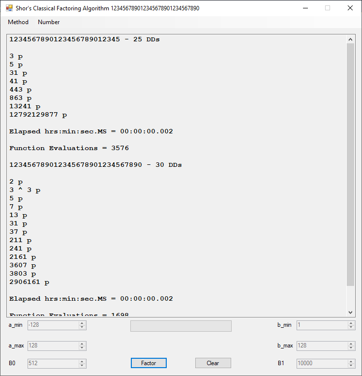
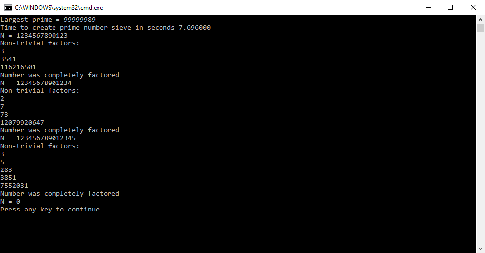
I implemented this algorithm for C long (32-bit) number in 1997, C# big integers in approximately 2015 or 2016, and C unsigned long long (64-bit) integers in March, 2023.
/*
Author: Pate Williams (c) 1997 - 2023
"Algorithm 8.1.1 (Trial Division). We assume given
a table of prime numbers p[1] = 2, p[2] = 3,..., p[k],
with k > 3, an array t <- [6, 4, 2, 4, 4, 6, 2], and
an index j such that if p[k] mod 30 is equal to
1, 7, 11, 13, 17, 19, 23 or 29 then j is equal to
0, 1, 2, 3, 4, 5, 6 or 7 respectively. Finally, we
give ourselves an upper bound B such that B >= p[k],
essentially to avoid spending too much time. Then
given a positive integer N, this algorithm tries to
factor (or split N) and if it fails, N will be free
of prime factors less than or equal to B."
-Henri Cohen-
See "A Course in Computational Algebraic Number
Theory" by Henri Cohen page 420.
*/
#include <math.h>
#include <stdio.h>
#include <stdlib.h>
#include <string.h>
#include <time.h>
#define BITS_PER_LONG 32
#define BITS_PER_LONG_1 31
#define MAX_SIEVE 100000000L
#define LARGEST_PRIME 99999989L
#define SIEVE_SIZE (MAX_SIEVE / BITS_PER_LONG)
typedef unsigned long long ull;
struct factor { int expon; ull prime; };
long *prime, sieve[SIEVE_SIZE];
int get_bit(long i, long *sieve) {
long b = i % BITS_PER_LONG;
long c = i / BITS_PER_LONG;
return (sieve[c] >> (BITS_PER_LONG_1 - b)) & 1;
}
void set_bit(long i, long v, long *sieve) {
long b = i % BITS_PER_LONG;
long c = i / BITS_PER_LONG;
long mask = 1 << (BITS_PER_LONG_1 - b);
if (v == 1)
sieve[c] |= mask;
else
sieve[c] &= ~mask;
}
void Sieve(long n, long *sieve) {
int c, i, inc;
set_bit(0, 0, sieve);
set_bit(1, 0, sieve);
set_bit(2, 1, sieve);
for (i = 3; i <= n; i++)
set_bit(i, i & 1, sieve);
c = 3;
do {
i = c * c, inc = c + c;
while (i <= n) {
set_bit(i, 0, sieve);
i += inc;
}
c += 2;
while (!get_bit(c, sieve)) c++;
} while (c * c <= n);
}
void get_bits(ull b, int *number, int *bits) {
int i = 0;
do {
bits[i++] = b % 2;
b = b / 2;
} while (b > 0);
*number = i;
}
ull pow_mod(
ull x,
ull b,
ull n) {
// Figure 4.4 in "Cryptography Theory and Practice"
// by Douglas R. Stinson page 127
int bits[64], i, l;
ull z = 1, s = 0;
get_bits(b, &l, bits);
s = bits[l - 1];
for (i = l - 2; i >= 0; i--)
s = 2 * s + bits[i];
if (b != s) {
printf("Error in pow_mod function\n");
exit(-1);
}
for (i = l - 1; i >= 0; i--) {
z = (z * z) % n;
if (bits[i] == 1)
z = (z * x) % n;
}
return z;
}
ull rand_ull(void) {
ull r = 0;
for (int i = 0; i < 64; i += 15 /*30*/) {
r = r * ((ull)RAND_MAX + 1) + rand();
}
return r;
}
int Miller_Rabin(ull n, int t) {
// returns 1 for prime
// returns 0 for composite
// "Handbook of Applied Cryptography"
// Alfred J. Menezes among others
// 4.24 Algorithm page 139
int i, j, s = 0;
ull a, n1 = n - 1, r, y;
r = n1;
while ((r % 2) == 0) {
s++;
r /= 2;
}
for (i = 0; i < t; i++)
{
while (true)
{
a = rand_ull() % n;
if (a >= 2 && a <= n - 2)
break;
}
y = pow_mod(a, r, n);
if (y != 1 && y != n1) {
j = 1;
while (j <= s - 1 && y != n1) {
y = (y * y) % n;
if (y == 1)
return 0;
j++;
}
if (y == n1)
return 0;
}
}
return 1;
}
int trial_division(ull *N, long *prime,
struct factor *f, int *count) {
int found;
ull B, d;
int e, i, j = 0, k, m, n;
int t[8] = { 6, 4, 2, 4, 2, 4, 6, 2 };
int table[8] = { 1, 7, 11, 13, 17, 19, 23, 29 };
ull l, r;
if (*N <= 5) {
*count = 1;
f[0].expon = 1;
switch (*N) {
case 1: f[0].prime = 1; break;
case 2: f[0].prime = 2; break;
case 3: f[0].prime = 3; break;
case 4: f[0].expon = 2; f[0].prime = 2; break;
case 5: f[0].prime = 5; break;
}
return 1;
}
*count = 0;
B = LARGEST_PRIME;
i = -1, l = (ull)sqrt((double)*N), m = -1;
L2:
m++;
if (i == MAX_SIEVE) {
i = j - 1;
goto L5;
}
d = prime[m];
k = d % 30;
found = 0;
for (n = 0; !found && n < 8; n++) {
found = k == table[n];
if (found) j = n;
}
L3:
r = *N % d;
if (r == 0) {
e = 0;
do {
e++;
*N /= d;
} while (*N % d == 0);
f[*count].expon = e;
f[*count].prime = d;
*count = *count + 1;
if (*N == 1) return 1;
goto L2;
}
if (d >= l) {
if (*N > 1) {
f[*count].expon = 1;
f[*count].prime = *N;
*count = *count + 1;
*N = 1;
return 1;
}
}
else if (i < 0) goto L2;
L5:
i = (i + 1) % 8;
d = d + t[i];
if (d > B) return 0;
goto L3;
}
int main(void) {
char e_buffer[256], n_buffer[256] = { 0 };
long k, e_length, n_length = 0, valid;
double time_spent;
int count;
long i, p = 2;
ull largest_prime;
long prime_count = 0;
ull N, sqrtN;
struct factor f[32];
clock_t begin, end;
begin = clock();
Sieve(MAX_SIEVE, sieve);
for (p = 2; p < MAX_SIEVE; p++) {
while (!get_bit(p, sieve))
p++;
prime_count++;
}
prime_count--;
prime = (long*)malloc(prime_count * sizeof(long));
i = 0;
p = 2;
while (i < prime_count)
{
while (!get_bit(p, sieve))
p++;
prime[i++] = p++;
}
largest_prime = LARGEST_PRIME;
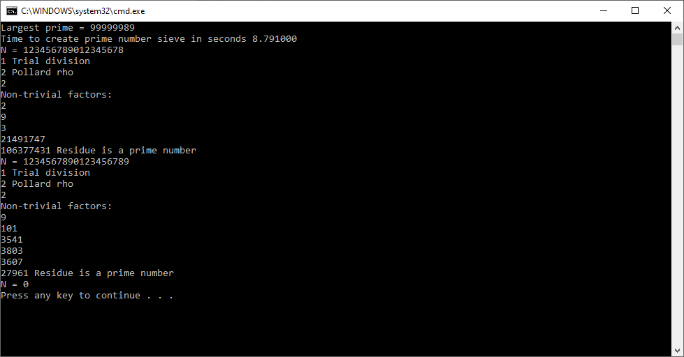
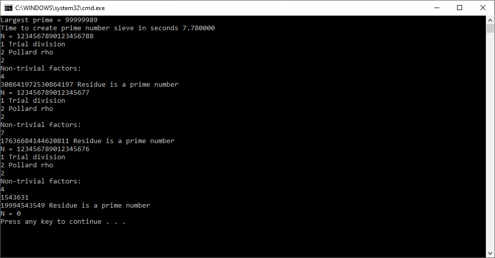
printf("Largest prime = %I64u\n", largest_prime);
end = clock();
time_spent = (double)(end - begin) / CLOCKS_PER_SEC;
printf("Time to create prime number sieve in seconds %lf\n", time_spent);
for (;;) {
printf("N = ");
scanf_s("%s", e_buffer, 256);
e_length = strlen(e_buffer);
n_length = 0;
valid = 1;
for (k = 0; valid && k < e_length; k++) {
if (e_buffer[k] >= '0' &&
e_buffer[k] <= '9' ||
e_buffer[k] == ',') {
if (e_buffer[k] != ',') {
n_buffer[n_length++] = e_buffer[k];
}
}
else {
valid = 0;
}
}
if (!valid) {
printf("Invalid character must in set {0, 1, ..., 9, ',')\n");
continue;
}
else {
n_buffer[n_length] = '\0';
N = atoll(n_buffer);
sqrtN = (ull)sqrt((double)N);
if (sqrtN > largest_prime) {
printf("Number is too large!\n");
printf("Square root %I64u must be < %I64u\n", sqrtN, largest_prime);
continue;
}
}
if (N <= 0) break;
trial_division(&N, prime, f, &count);
printf("Non-trivial factors:\n");
for (i = 0; i < count; i++) {
printf("%I64u", f[i].prime);
if (f[i].expon > 1) printf(" ^ %ld\n", f[i].expon);
else printf("\n");
}
if (N != 1)
{
if (Miller_Rabin(N, 20) == 1)
printf("Residue is a prime number\n");
else
printf("Last factor is composite\n");
}
else
printf("Number was completely factored\n");
}
return 0;
}