Computation of Ulam Primes in C++ Translation from Python by James Pate Williams, Jr (c) 2008 – 2023.

http://en.wikipedia.org/wiki/Ulam_numbers

https://oeis.org/A002858

Stanislaw Marcin Ulam worked on the Manhattan Project by an invitation from John von Neumann:

https://en.wikipedia.org/wiki/Stanis%C5%82aw_Ulam#Move_to_the_United_States

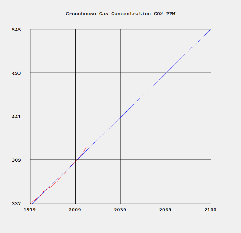
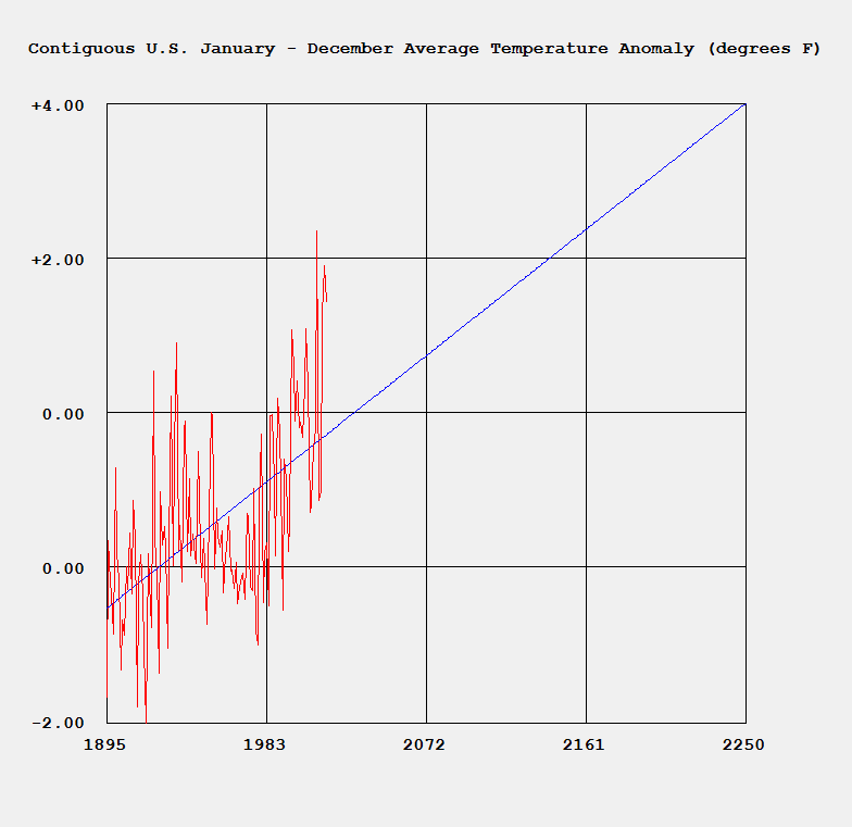
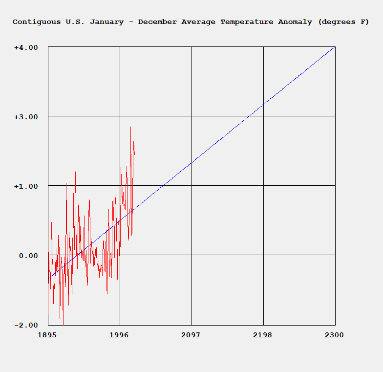
Ulam is given credit for the Teller-Ulam design of the hydrogen bomb. Edward Teller was one of the first proponent of human induced global climate change:

https://en.wikipedia.org/wiki/Edward_Teller#Hydrogen_bomb

/*
	Translator: James Pate Williams, Jr. (c) 2008

	Translated to C++ from the following python code:

	http://en.wikipedia.org/wiki/Ulam_numbers
	https://oeis.org/A002858

	ulam_i = [1,2,3]
	ulam_j = [1,2,3]
	for cand in range(4,5000):
		res = []
		for i in ulam_i:
			for j in ulam_j:
				if i == j or j > i: pass
				else:
					res.append(i+j)
				if res.count(cand) == 1:
				ulam_i.append(cand)
				ulam_j.append(cand)
			print ulam_i

	Find the Ulam primes <= 5000
*/

#include "stdafx.h"
#include <time.h>
#include <iomanip>
#include <iostream>
#include <vector>
using namespace std;

bool sieve[10000000];

void PopulateSieve(bool *sieve, int number) {

	// sieve of Eratosthenes

	int c, inc, i, n = number - 1;

	for (i = 0; i < n; i++)
		sieve[i] = false;

	sieve[1] = false;
	sieve[2] = true;

	for (i = 3; i <= n; i++)
		sieve[i] = (i & 1) == 1 ? true : false;

	c = 3;

	do {
		i = c * c;
		inc = c + c;

		while (i <= n) {
			sieve[i] = false;
			i += inc;
		}

		c += 2;
		while (!sieve[c])
			c++;
	} while (c * c <= n);
}

bool CountEqualOne(int number, vector<int> ulam) {
	int count = 0, i;

	for (i = 0; i < ulam.size(); i++)
		if (ulam[i] == number)
			count++;

	return count == 1;
}

void UlamNumbers(int n) {
	int candidate, i, j;
	vector<int> vI;
	vector<int> vJ;
	vector<int> UlamResult;

	PopulateSieve(sieve, 10000000);

	for (i = 1; i <= 3; i++) {
		vI.push_back(i);
		vJ.push_back(i);
	}

	for (candidate = 4; candidate <= n; candidate++) {

		UlamResult.clear();

		for (i = 0; i < vI.size(); i++) {
			int ui = vI[i];

			for (j = 0; j < vJ.size(); j++) {
				int uj = vJ[j];

				if (ui == uj || uj > ui)
					continue;

				UlamResult.push_back(ui + uj);
			}
		}

		if (CountEqualOne(candidate, UlamResult)) {
			vI.push_back(candidate);
			vJ.push_back(candidate);
		}
	}

	j = 0;

	for (i = 0; i < vI.size(); i++) {
		if (sieve[vI[i]]) {
			cout << setw(4) << vI[i] << ' ';

			if ((j + 1) % 10 == 0) {
				j = 0;
				cout << endl;
			}
			else
				j++;
		}
	}

	cout << endl;
}

int main(int argc, char * const argv[]) {
	clock_t clock0 = clock();

	cout << "Ulam sequence prime numbers < 5000" << endl << endl;
	UlamNumbers(5000);
	clock0 = clock() - clock0;
	cout << endl << endl << "seconds = ";
	cout << (double)clock0 / CLOCKS_PER_SEC << endl;
	return 0;
}

Georgia Climate Data by James Pate Williams, Jr.

Abstract

I became interested in attempting to predict temperatures in the state of Georgia way back in the day, i.e., the date was November 1 – 4, 2009. I found a neat website for the temperatures from January 1895 to December 2001. Unfortunately, the website no longer exists online, however, I saved the data to an extinct PC of mine and a USB solid state drive. I used two methods to attempt predictions of the annual temperatures from January 2002 to December 2025. The first algorithm is polynomial least squares curve fitting [1]. The second method is a radial basis function neural network [2] [3] that is trained by an evolutionary hill-climber of my design and implementation [4] [5]. The applications were written in one of my favorite computer programming languages, namely, C# [6].

Methodologies

I created a polynomial least squares dynamic-link library (DLL) using Gaussian elimination with pivoting and an inverse matrix calculation utilizing an upper-triangular matrix [7]. At first the driver application was capable of fitting a 1-degree to 100-degrees polynomial. I found that my algorithm was only valid for a 1-degree to 76-degrees fitting polynomial. I used degrees: 1, 4, 8, 16, 32, 64, and 76.

Predicted Statewide Georgia Annual Average Temperatures in Degrees Fahrenheit
Poly Degree14816326476Model
YearT (F)T (F)T (F)T (F)T (F)T (F)T (F)Average
200264.263.163.863.662.463.062.963.3
200364.263.263.663.464.163.763.763.7
200464.263.363.463.464.563.964.063.8
200564.263.363.463.564.263.964.063.8
200664.263.463.463.663.863.763.863.7
200764.263.563.463.763.363.663.663.6
200864.263.663.463.763.063.463.463.5
200964.263.663.463.762.963.363.363.5
201064.163.763.563.762.963.363.263.5
201164.163.863.663.663.163.363.263.5
201264.163.863.763.663.363.463.363.6
201364.163.963.763.663.663.563.563.7
201464.163.963.863.663.963.663.663.8
201564.164.063.963.664.163.863.863.9
201664.164.063.963.664.363.963.964.0
201764.164.164.063.764.464.064.164.1
201864.164.164.163.764.464.164.264.1
201964.164.264.163.964.464.264.264.2
202064.164.264.264.064.364.364.364.2
202164.164.364.264.164.264.364.364.2
202264.164.364.264.264.264.364.364.2
202364.164.364.364.364.164.364.364.2
202464.064.464.364.564.064.364.364.3
202564.064.464.364.664.064.364.364.3

The second method was a radial basis function neural network that was trained by an evolutionary hill-climber of my design and implementation. I used 8, 16, 32, 64 basis functions. The population of the hill-climber was 16 and generations 262,144.

Predicted Statewide Georgia Annual Average Temperatures in Degrees Fahrenheit
Basis8163264Model
YearT (F)T (F)T (F)T (F)Average
200265.464.265.465.265.1
200365.564.265.465.265.1
200465.564.265.565.365.1
200565.564.265.565.365.1
200665.664.265.565.365.2
200765.664.265.665.365.2
200865.664.265.665.465.2
200965.764.265.665.465.2
201065.764.265.665.465.2
201165.764.265.765.465.3
201265.764.265.765.565.3
201365.864.265.765.565.3
201465.864.265.865.565.3
201565.864.365.865.565.4
201665.964.365.865.665.4
201765.964.365.865.665.4
201865.964.365.965.665.4
201966.064.365.965.665.5
202066.064.365.965.765.5
202166.064.366.065.765.5
202266.064.366.065.765.5
202366.164.366.065.765.5
202466.164.366.165.865.6
202566.164.366.165.865.6

I trust the polynomial fitting results more than the radial basis function neural network values. The polynomial fitting had mean square errors < 1 whereas the radial basis function neural network had mean square errors between 1 and 9. The general trends were increasing temperatures which are in line with the theorized global warming.

References

[1]H. T. Lau, A Numerical Library in C for Scientists and Engineers, Boca Raton: CRC Press, 1995.
[2]T. M. Mitchell, Machine Learning, Boston: WCB McGraw-Hill, 1997.
[3]A. P. Engelbrecht, Computational Intelligence An Introduction, Hoboken: John Wiley and Sons, 2002.
[4]Z. Michalewicz, Genetic Algorithms + Data Structures = Evolutionary Programs 3rd Edition, Berlin: Springer, 1999.
[5]D. B. Fogel, Evolutionary Computation Toward a New Philosophy of Machine Intelligence, Piscataway: IEEE Press, 2000.
[6]C. Petzold, Programming Windows with C#, Redmond: Microsoft Press, 2002.
[7]S. D. Conte and C. d. Boor, Elementary Numerical An Algorithmic Approach, New York: McGraw-Hill Book Company, 1980.

Global Primary Greenhouse Gas Concentrations by James Pate Williams Jr BA, BS, MSwE, PhD

I designed and implemented a C# computer language application to model the global greenhouse gas concentrations data found on the NOAA website:

https://www.esrl.noaa.gov/gmd/aggi/aggi.html

I used the latest recommended data for time period 1979 to 2017. The concentrations of three greenhouse gases were modeled: carbon dioxide (CO2), methane (CH4), and nitrous oxide (N2O).

The empirical modeling paradigm I used was simple linear regression. My model goes out to the year 2300. The key formulas used by the model are:

                                Simple Linear Regression Parameters

See the website:

https://en.wikipedia.org/wiki/Simple_linear_regression

Some plots of the concentrations in parts per million (PPM) and parts per billion (PPB) are given below.

                                                Carbon Dioxide Concentration in Parts Per Million
                                                        Methane Concentration in Parts Per Billion
                                                 Nitrous Oxide Concentration in Parts Per Billion
                                             Carbon Dioxide Concentration in Parts Per Million
                                                      Methane Concentration in Parts Per Billion
                                                   Nitrous Oxide Concentration in Parts Per Billion
              Simple Linear Regression Parameters
              Simple Linear Regression Parameters
             Simple Linear Regression Parameters
                                                         Greenhouse Gas Concentrations Table

NOAA Contiguous United States of America Precipitation by James Pate Williams Jr BA, BS, MSwE, PhD

I designed and implemented a C# computer language application to model the precipitation data found on the NOAA website:

https://www.ncdc.noaa.gov

I used the latest recommended data for time period 1895 to 2017. The empirical modeling paradigm I used was simple linear regression. My model goes out to the year 2300. The key formulas used by the model are:

Simple  Linear Regression Equations

See the website:

https://en.wikipedia.org/wiki/Simple_linear_regression

Some plots of the contiguous U.S. precipitation are shown below. The climate is getting wetter thus some parts of the U.S.maybe more prone to floods.

Precipitation Plot
Precipitation Plot
Precipitation Plot
Precipitation Plot
Precipitation Plot
Precipitation Plot
Precipitation Plot
Simple Linear Regression Parameters
Precipitation Table Experimental and Theoretical Values

NOAA Contiguous United States of America Temperature Anomaly by James Pate Williams Jr BA, BS, MSwE, PhD

I designed and implemented a C# computer language application to model the temperature anomaly data found on the NOAA website:

https://www.ncdc.noaa.gov

I used the latest recommended data for time period 1895 to 2017. The empirical modeling paradigm I used was simple linear regression. My model goes out to the year 2300. The key formulas used by the model are:

Simple Linear Regression Equations

See the website:

https://en.wikipedia.org/wiki/Simple_linear_regression

Below are some plots of the temperature anomaly.

Temperature Anomaly Actual Anomaly in Red Theoretical in Blue
C# Application Main Form
Simple Linear Regression Parameters
Table Function Form with Experimental and Theoretical Anomalies