Category: Computer Science
Complex Number Calculator © March 25-26 by James Pate Williams, Jr.
New 1d Integration Results (c) March 24, 2024, by James Pate Williams, Jr.
I tested NUMAL’s integration function versus homegrown trapezoidal rule and Simpson’s rule. The second and third algorithms were closed (included both endpoints). There exist higher order Newton-Cotes integration formulas. I did not test the Gauss-Legendre and/or Gauss-Laguerre integration method(s). The trapezoidal rule can be improved if the derivative of the integrand is known and is easily calculated.
C Sorting DLL Experimental Results by James Pate Williams, Jr. (c) March 22, 2024, All Applicable Rights Reserved
Microsoft Visual Studio 2019 Community Version – Creating and Using a C Based Dynamic Link Library © March 22, 2024, by James Pate Williams, Jr.
Create a solution using the DLL C++ DLL template. Rename pch.cpp to pch.c and dllmain.cpp to dllmain.c. Add a header file for the DLL containing the following macro:
#define DLL_Export __declspec(dllexport)
Mark all the exportable functions in the DLL header file with the DLL_Export macro. Suppose the DLL is named CSortingDLL. Next create a console C++ project in the DLL solution to use the DLL. Open the Properties page of the console app. If you want to use the ASCII character set, select the Advanced Configuration Properties, and set the Character Set to Not Set. Now open the C/C++ General Property and under Additional Include Directories add ..\CSortingDLL\;. Do not include the previous period mark. Next open the Linker General Property page. Set Additional Library Directories to ..\CSortingDLL\$(IntDir);. The penultimate step is to set the Linker Input Additional Dependencies to CSortingDLL.lib;. The final step for the app is to add a reference to CSortingDLL. Now you have a functioning DLL and an app using the DLL. If you have any questions, please contact me via email at jamespate@mac.com. Also, Microsoft has a DLL walkthrough complete with source code. I will add my CSortingDLL header source code as a PDF document.
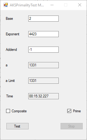
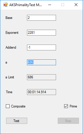
BigInteger Multitasking Agrawal, Kayal, and Saxena (AKS) Primality Test (c) June 19, 2016, by James Pate Williams, Jr. Microsoft TechNet Project Description
This application implements the algorithm described in the paper at the URL http://www.cse.iitk.ac.in/users/manindra/algebra/primality_v6.pdf. I replaced Step 1 of the algorithm with the Miller-Rabin probabilistic primality test. If that test shows that the number is composite, I return the value COMPOSITE. This algorithm is much easier to implement and understand that Wieb Bosmer’s Primality Proving with Cyclotomy also known as the Jacobi sums primality test. As a test we determine that the following Mersenne numbers are prime: M_1279, M_2203, M_2281, M_3217, and M_4253 where M_n = 2 ^ n – 1, and the primes have 386, 664, 687, 969, and 1281 decimal digits, respectively. M_1279 was first proven prime by Raphael M. Robinson on June 25, 1952, using the Lucas-Lehmer test on a SWAC computer. The same author found that M_2203 was prime on October 7, 1952, and M_2281 was prime on October 9, 1952, using the same method and computer. Hans Riesel determined that M_3217 was prime on September 8, 1957, using the Lucas-Lehmer test on a BESK computer. M_4253 was proven prime on November 3, 1961 by Alexander Hurwitz using the Lucas-Lehmer test on an IBM 7090 mainframe computer. See http://www.mersenne.org/primes/ for many more Mersenne primes. All of the computations illustrated below were performed on a late November 2015 Dell XPS 8900 computer with 16 GB RAM Intel(R) Core(TM) i7-6700K CPU @ 4.00 GHz running Windows 10 Pro. The .Net framework is .Net 4.5.2. This is a multitasking version of the original BigInteger variant of the application. Someone with a quad core CPU with 8 virtual processors can try NumberTasks = 8 to see if that speeds up this application more or less. I usually try to limit the number of tasks to actual number of cores.


Preliminary Factorization Results of the Thirteenth Fermat Number (c) February 5, 2024, by James Pate Williams, Jr.
I am working on a factorization of the Thirteenth Fermat number which is 2 ^ 8192 + 1 and is 2,467 decimal digits in length. I am using Pollard’s factoring with cubic integers on the number (2 ^ 2731) ^ 3 + 2. I am also utilizing a homegrown variant of the venerable Pollard and Brent rho method and Arjen K. Lenstra’s Free LIP Elliptic Curve Method. I can factor the seventh Fermat number 2 ^ 128 + 1 in five to thirty minutes using my C# code. The factoring with cubic integers code is in C and uses Free-LIP.
Fermat factoring status (prothsearch.com)
The following is a run of Lenstra’s ECM algorithm:
== Data Menu ==
1 Simple Number
2 Fibonacci Sequence Number
3 Lucas Sequence Number
4 Exit
Enter option (1 – 4): 1
Enter a number to be factored: 2^8192+1
Enter a random number generator seed: 1
== Factoring Menu ==
1 Lenstra’s ECM
2 Lenstra’s Pollard-Rho
3 Pollard’s Factoring with Cubic Integers
Option (1 – 3): 1
2710954639361 p # digits 13
3603109844542291969 p # digits 19
Runtime (s) = 17015.344000
I aborted the previous computation due to the fact I was curious about the number of prime factors that could be found on personal computer. I will try a lot more calculation time in a future run. My homegrown application is able to at least find the first factor of Fermat Number 13.
Latest Factoring Results (c) February 4, 2024, by James Pate Williams, Jr.
I am testing two factoring algorithms: Pollard-Shor-Williams’s method, a home-grown version of the venerable Pollard rho algorithm and Pollard’s factoring with cubic integers. The second recipe is from “The Development of the Number Field Sieve” edited by Arjen K. Lenstra and Hendrik W. Lenstra, Jr. I use the 20-digit test number, 2 ^ 66 + 2 = 73786976294838206466. My method is very fast with this number as shown below:
2^66+2
73786976294838206466 20
Pseudo-Random Number Generator Seed = 1
Number of Tasks = 1
2 p 1
3 p 1
11 p 2
131 p 3
2731 p 4
409891 p 6
7623851 p 7
Elapsed hrs:min:sec.MS = 00:00:00.652
Function Evaluations = 1995
The Pollard factoring with cubic integers takes a long time but is capable of factoring much larger numbers. The results of the full factorization of my test number are:
== Data Menu ==
1 Simple Number
2 Fibonacci Sequence Number
3 Lucas Sequence Number
4 Exit
Enter option (1 – 4): 1
Enter a number to be factored: 2^66+2
Enter a random number generator seed: 1
== Factoring Menu ==
1 Lenstra’s ECM
2 Lenstra’s Pollard-Rho
3 Pollard’s Factoring with Cubic Integers
Option (1 – 3): 3
73786976294838206466
Enter a lower bound : -50000
Enter a upper bound : +50000
Enter b lower bound : +1
Enter b upper bound : +50000
Enter maximum kernels : 1024
Enter algebraic prime count: 300
Enter rational prime count: 300
Enter lo large prime bound: 10000
Enter hi large prime bound: 11000
Numbers sieved = 452239293
Successes 0 gcd(a, b) is 1 = 274929004
Successes 1 rational smooth a + b * r = 181838258
Successes 2 long long smooth = 68959
Successes 3 kernels tested = 535
2 p # digits 1
3 p # digits 1
11 p # digits 2
131 p # digits 3
2731 p # digits 4
409891 p # digits 6
7623851 p # digits 7
Runtime (s) = 36383.696000
It took over ten hours to fully factor, 2 ^ 66 + 2. I am currently attempting to factor the Thirteenth Fermat number which is 2 ^ (2 ^ 13) + 1 = 2 ^ 8192 + 1. The number has 2,467 decimal digits. I am using 399 algebraic prime numbers, 600 rational prime numbers, and 316 “large prime numbers” (primes between 12,000 and 15,000). I have to find the kernels of a 1316 by 1315 matrix. I am trying the factorization using a maximum of 8192 kernels. I suspect this computation will take about a week on my desktop workstation. There is no guarantee that I will find a non-trivial factor of 2 * (2731 ^ 3) + 2.
