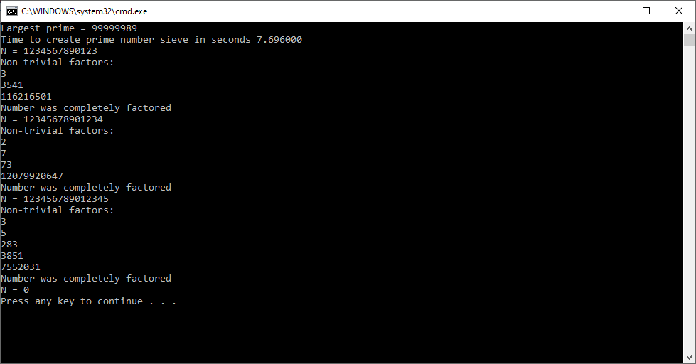
See the following website for the used algorithms pages 119 to 121:


See the following website for the used algorithms pages 119 to 121:
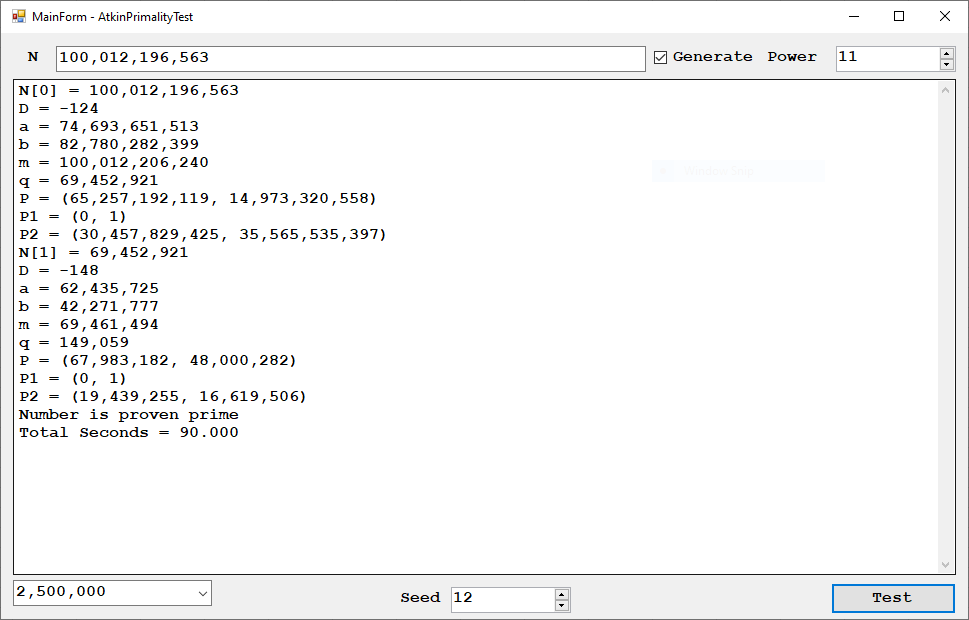
Back in 2022 I reimplemented Henri Cohen’s Atkin’s Primality Test algorithm. This test makes use of an elliptic curve analog of Pocklington’s theorem. I restate the theorem utilized from Henri Cohen’s “A course in Computational Algebraic Number Theory” on pages 467 to 468: “Proposition 9.2.1. Let N be an integer coprime to 6 and different from 1, and E be an elliptic curve modulo N. Assume that we know an integer m a point P contained on the elliptic curve satisfying the following conditions. (1) There exists a prime divisor q of m such that q > (N^1/4 + 1) ^ 2 (2) m * P = O_E = (0 : 1 : ). (3) (m / q) * P = (x : y : t) with t contained in (Z/NZ)*. Then N is prime.” I used C# and Microsoft’s BigInteger class. I have not been able to prove numbers greater than 14 decimal digits to be prime. I am recoding the algorithm in C++ which limits me to 19 decimal digits since 2 ^ 63 – 1 = 9,223,372,036,854,775,807 (Int64).


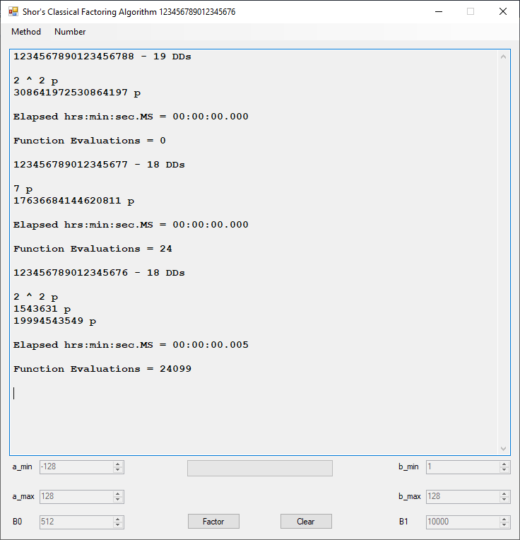
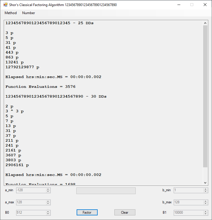
I implemented the algorithm in C using unsigned 64-bit integers. This method is good for integers of around 18 decimal digits in length. For comparison I tested against my blazingly fast Shor’s classical factoring algorithm which works on arbitrarily large integers of around 50 to 60 or more decimal digits.
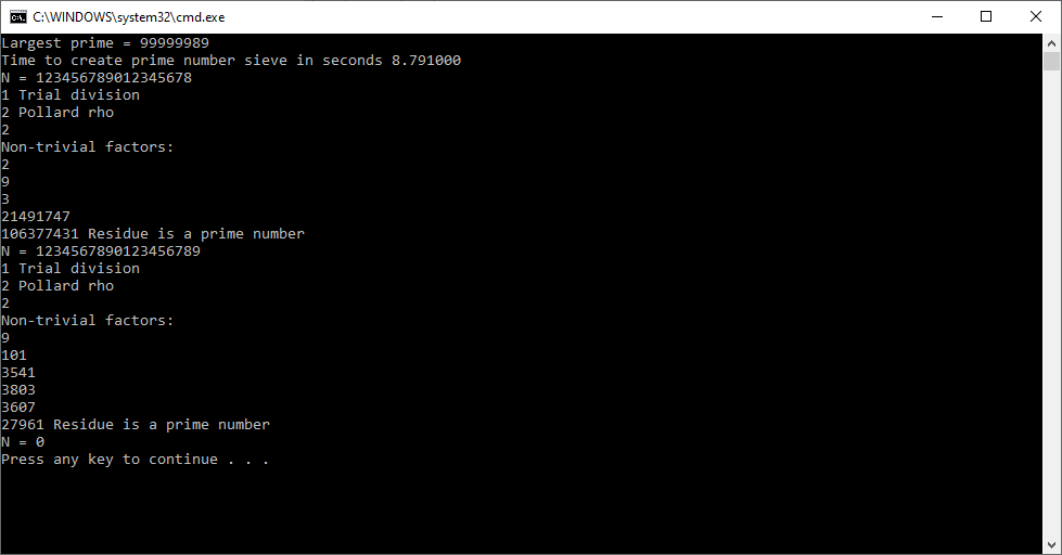
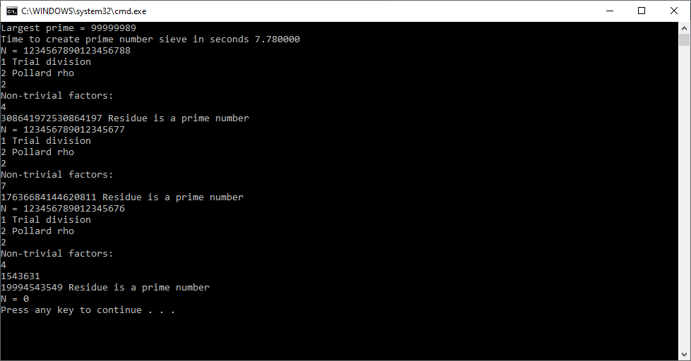
I implemented this algorithm for C long (32-bit) number in 1997, C# big integers in approximately 2015 or 2016, and C unsigned long long (64-bit) integers in March, 2023.

/*
Author:  Pate Williams (c) 1997 - 2023

"Algorithm 8.1.1 (Trial Division). We assume given
a table of prime numbers p[1] = 2, p[2] = 3,..., p[k],
with k > 3, an array t <- [6, 4, 2, 4, 4, 6, 2], and
an index j such that if p[k] mod 30 is equal to
1, 7, 11, 13, 17, 19, 23 or 29 then j is equal to
0, 1, 2, 3, 4, 5, 6 or 7 respectively. Finally, we
give ourselves an upper bound B such that B >= p[k],
essentially to avoid spending too much time. Then
given a positive integer N, this algorithm tries to
factor (or split N) and if it fails, N will be free
of prime factors less than or equal to B."
-Henri Cohen-
See "A Course in Computational Algebraic Number
Theory" by Henri Cohen page 420.
*/

#include <math.h>
#include <stdio.h>
#include <stdlib.h>
#include <string.h>
#include <time.h>

#define BITS_PER_LONG   32
#define BITS_PER_LONG_1 31
#define MAX_SIEVE 100000000L
#define LARGEST_PRIME 99999989L
#define SIEVE_SIZE (MAX_SIEVE / BITS_PER_LONG)

typedef unsigned long long ull;

struct factor { int expon;  ull prime; };
long *prime, sieve[SIEVE_SIZE];

int get_bit(long i, long *sieve) {
	long b = i % BITS_PER_LONG;
	long c = i / BITS_PER_LONG;

	return (sieve[c] >> (BITS_PER_LONG_1 - b)) & 1;
}

void set_bit(long i, long v, long *sieve) {
	long b = i % BITS_PER_LONG;
	long c = i / BITS_PER_LONG;
	long mask = 1 << (BITS_PER_LONG_1 - b);

	if (v == 1)
		sieve[c] |= mask;
	else
		sieve[c] &= ~mask;
}

void Sieve(long n, long *sieve) {
	int c, i, inc;

	set_bit(0, 0, sieve);
	set_bit(1, 0, sieve);
	set_bit(2, 1, sieve);
	for (i = 3; i <= n; i++)
		set_bit(i, i & 1, sieve);
	c = 3;
	do {
		i = c * c, inc = c + c;
		while (i <= n) {
			set_bit(i, 0, sieve);
			i += inc;
		}
		c += 2;
		while (!get_bit(c, sieve)) c++;
	} while (c * c <= n);
}

void get_bits(ull b, int *number, int *bits) {
	int i = 0;
	do {
		bits[i++] = b % 2;
		b = b / 2;
	} while (b > 0);
	*number = i;
}

 ull pow_mod(
	 ull x,
	 ull b,
	 ull n) {
	// Figure 4.4 in "Cryptography Theory and Practice"
	// by Douglas R. Stinson page 127
	int bits[64], i, l;
	ull z = 1, s = 0;

	get_bits(b, &l, bits);
	s = bits[l - 1];
	for (i = l - 2; i >= 0; i--)
		s = 2 * s + bits[i];
	if (b != s) {
		printf("Error in pow_mod function\n");
		exit(-1);
	}
	for (i = l - 1; i >= 0; i--) {
		z = (z * z) % n;
		if (bits[i] == 1)
			z = (z * x) % n;
	}
	return z;
}

ull rand_ull(void) {
	ull r = 0;
	for (int i = 0; i < 64; i += 15 /*30*/) {
		r = r * ((ull)RAND_MAX + 1) + rand();
	}
	return r;
}

int Miller_Rabin(ull n, int t) {
	// returns 1 for prime
	// returns 0 for composite
	// "Handbook of Applied Cryptography"
	// Alfred J. Menezes among others
	// 4.24 Algorithm page 139
	int i, j, s = 0;
	ull a, n1 = n - 1, r, y;

	r = n1;
	while ((r % 2) == 0) {
		s++;
		r /= 2;
	}
	for (i = 0; i < t; i++)
	{
		while (true)
		{
			a = rand_ull() % n;

			if (a >= 2 && a <= n - 2)
				break;
		}
		y = pow_mod(a, r, n);
		if (y != 1 && y != n1) {
			j = 1;
			while (j <= s - 1 && y != n1) {
				y = (y * y) % n;
				if (y == 1)
					return 0;
				j++;
			}
			if (y == n1)
				return 0;
		}
	}
	return 1;
}

int trial_division(ull *N, long *prime,
	struct factor *f, int *count) {
	int found;
	ull B, d;
	int e, i, j = 0, k, m, n;
	int t[8] = { 6, 4, 2, 4, 2, 4, 6, 2 };
	int table[8] = { 1, 7, 11, 13, 17, 19, 23, 29 };
	ull l, r;

	if (*N <= 5) {
		*count = 1;
		f[0].expon = 1;
		switch (*N) {
		case 1: f[0].prime = 1; break;
		case 2: f[0].prime = 2; break;
		case 3: f[0].prime = 3; break;
		case 4: f[0].expon = 2; f[0].prime = 2; break;
		case 5: f[0].prime = 5; break;
		}
		return 1;
	}
	*count = 0;
	B = LARGEST_PRIME;
	i = -1, l = (ull)sqrt((double)*N), m = -1;
L2:
	m++;
	if (i == MAX_SIEVE) {
		i = j - 1;
		goto L5;
	}
	d = prime[m];
	k = d % 30;
	found = 0;
	for (n = 0; !found && n < 8; n++) {
		found = k == table[n];
		if (found) j = n;
	}
L3:
	r = *N % d;
	if (r == 0) {
		e = 0;
		do {
			e++;
			*N /= d;
		} while (*N % d == 0);
		f[*count].expon = e;
		f[*count].prime = d;
		*count = *count + 1;
		if (*N == 1) return 1;
		goto L2;
	}
	if (d >= l) {
		if (*N > 1) {
			f[*count].expon = 1;
			f[*count].prime = *N;
			*count = *count + 1;
			*N = 1;
			return 1;
		}
	}
	else if (i < 0) goto L2;
L5:
	i = (i + 1) % 8;
	d = d + t[i];
	if (d > B) return 0;
	goto L3;
}

int main(void) {
	char e_buffer[256], n_buffer[256] = { 0 };
	long k, e_length, n_length = 0, valid;
	double time_spent;
	int count;
	long i, p = 2;
	ull largest_prime;
	long prime_count = 0;
	ull N, sqrtN;
	struct factor f[32];
	clock_t begin, end;

	begin = clock();
	Sieve(MAX_SIEVE, sieve);
	for (p = 2; p < MAX_SIEVE; p++) {
		while (!get_bit(p, sieve))
			p++;
		prime_count++;
	}
	prime_count--;
	prime = (long*)malloc(prime_count * sizeof(long));
	i = 0;
	p = 2;
	while (i < prime_count)
	{
		while (!get_bit(p, sieve))
			p++;
		prime[i++] = p++;
	}
	largest_prime = LARGEST_PRIME;
	printf("Largest prime = %I64u\n", largest_prime);
	end = clock();
	time_spent = (double)(end - begin) / CLOCKS_PER_SEC;
	printf("Time to create prime number sieve in seconds %lf\n", time_spent);
	for (;;) {
		printf("N = ");
		scanf_s("%s", e_buffer, 256);
		e_length = strlen(e_buffer);
		n_length = 0;
		valid = 1;
		for (k = 0; valid && k < e_length; k++) {
			if (e_buffer[k] >= '0' &&
				e_buffer[k] <= '9' ||
				e_buffer[k] == ',') {
				if (e_buffer[k] != ',') {
					n_buffer[n_length++] = e_buffer[k];
				}
			}
			else {
				valid = 0;
			}
		}
		if (!valid) {
			printf("Invalid character must in set {0, 1, ..., 9, ',')\n");
			continue;
		}
		else {
			n_buffer[n_length] = '\0';
			N = atoll(n_buffer);
			sqrtN = (ull)sqrt((double)N);
			if (sqrtN > largest_prime) {
				printf("Number is too large!\n");
				printf("Square root %I64u must be < %I64u\n", sqrtN, largest_prime);
				continue;
			}
		}
		if (N <= 0) break;
		trial_division(&N, prime, f, &count);
		printf("Non-trivial factors:\n");
		for (i = 0; i < count; i++) {
			printf("%I64u", f[i].prime);
			if (f[i].expon > 1) printf(" ^ %ld\n", f[i].expon);
			else printf("\n");
		}
		if (N != 1)
		{
			if (Miller_Rabin(N, 20) == 1)
				printf("Residue is a prime number\n");
			else
				printf("Last factor is composite\n");
		}
		else
			printf("Number was completely factored\n");
	}
	return 0;
}
/*
Author: Pate Williams (c) January 22, 1995
The following program is a translation of the FORTRAN
subprogram found in Elementary Numerical Analysis by
S. D. Conte and Carl de Boor pages 343-344. The program
uses Romberg extrapolation to find the integral of a
function.
*/
#include "stdafx.h"
#include <math.h>
#include <stdlib.h>
#include <time.h>
#include <stdio.h>
typedef long double real;
real t[10][10];
real f(real x)
{
return(expl(-x * x));
}
real Li(real x)
{
return(1.0 / logl(x));
}
real romberg(
real a, real b, int start, int row,
real(*f)(real))
{
int i, k, m;
real h, ratio, sum;
m = start;
h = (b - a) / m;
sum = 0.5 * (f(a) + f(b));
if (m > 1)
for (i = 1; i < m; i++)
sum += f(a + i * h);
t[1][1] = h * sum;
if (row < 2) return(t[1][1]);
for (k = 2; k <= row; k++)
{
h = 0.5 * h;
m *= 2;
sum = 0.0;
for (i = 1; i <= m; i += 2)
sum += f(a + h * i);
t[k][1] = 0.5 * t[k - 1][1] + sum * h;
for (i = 1; i < k; i++)
{
t[k - 1][i] = t[k][i] - t[k - 1][i];
t[k][i + 1] = t[k][i] - t[k - 1][i] /
(powl(4.0, (real)i) - 1.0);
}
}
if (row < 3) return(t[2][2]);
for (k = 1; k <= row - 2; k++)
for (i = 1; i <= k; i++)
{
if (t[k + 1][i] == 0.0)
ratio = 0.0;
else
ratio = t[k][i] / t[k + 1][i];
t[k][i] = ratio;
}
return(t[row][row - 1]);
}
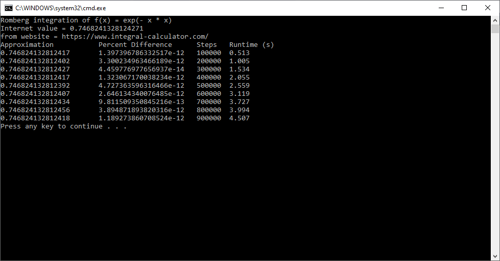
int main(void)
{
long double experimental = 0.7468241328124271;
int row = 8;
printf("first test\n");
printf("Romberg integration of f(x) = exp(- x * x)\n");
printf("Internet value = 0.7468241328124271\n");
printf("from website = https://www.integral-calculator.com/\n");
printf("Approximation\t\tPercent Difference\tSteps\tRuntime (s)\n");
for (long steps = 100000; steps <= 900000; steps += 100000)
{
clock_t start = clock();
long double trial = romberg(0.0, 1.0, steps, row, f);
clock_t endTm = clock();
long double runtime = ((long double)endTm - start) /
CLOCKS_PER_SEC;
long double pd = 100.0 * fabsl(experimental - trial) /
(0.5 *(experimental + trial));
printf("%16.15lf\t%16.15le\t%6d\t%4.3lf\n",
trial, pd, steps, runtime);
}
printf("second test\n");
printf("Romberg integration of Li(x) = 1 / ln x between 2 and some n\n");
printf("approximates the number of prime numbers between 2 and n\n");
printf("n\t\tLi(n)\t\tSteps\tTime (s)\n");
for (long n = 10; n <= 1000000000; n *= 10)
{
long steps = 1000000;
clock_t start = clock();
long double trial = romberg(2.0, n, steps, row, Li);
clock_t endTm = clock();
long double runtime = ((long double)endTm - start) /
CLOCKS_PER_SEC;
printf("%12ld\t%12.0lf\t%7ld\t%4.3lf\n",
n, trial, steps, runtime);
}
return(0);
}

/*
Author:  Pate Williams (c) January 20, 1995
The following is a translation of the Pascal program
sieve found in Pascalgorithms by Edwin D. Reilly and
Francis D. Federighi page 652. This program uses sets
to represent the sieve (see C Programming Language An
Applied Perspective by Lawrence Miller and Alec Qui-
lici pages 160 - 162).
*/
#include "stdafx.h"
#include <math.h>
#include <stdio.h>
#include <time.h>

#define _WORD_SIZE 32
#define _VECT_SIZE 31250000
#define SET_MIN    0
#define SET_MAX    1000000000

typedef long LONG;
typedef long SET[_VECT_SIZE];
typedef LONG ELEMENT;

SET set;

static LONG get_bit_pos(LONG *long_ptr, LONG *bit_ptr,
	ELEMENT element)
{
	*long_ptr = element / _WORD_SIZE;
	*bit_ptr = element % _WORD_SIZE;
	return(element >= SET_MIN && element <= SET_MAX);
}

static void set_bit(ELEMENT element, LONG inset)
{
	LONG bit, word;

	if (get_bit_pos(&word, &bit, element))
		inset ? set[word] |= (01 << bit) :
		set[word] &= ~(01 << bit);
}

static int get_bit(ELEMENT element)
{
	LONG bit, word;

	return(get_bit_pos(&word, &bit, element) ?
		(set[word] >> bit) & 01 : 0);
}

void set_Add(ELEMENT element)
{
	set_bit(element, 1);
}

void set_Del(ELEMENT element)
{
	set_bit(element, 0);
}

int set_Mem(ELEMENT element)
{
	return get_bit(element);
}

void primes(LONG n)
{
	LONG c, i, inc, k;
	double x;

	clock_t now = clock();
	set_Add(2);
	for (i = 3; i <= n; i++)
		if ((i + 1) % 2 == 0)
			set_Add(i);
		else
			set_Del(i);
	c = 3;
	do
	{
		i = c * c;
		inc = c + c;
		while (i <= n)
		{
			set_Del(i);
			i = i + inc;
		}
		c += 2;
		while (set_Mem(c) == 0) c += 1;
	} while (c * c <= n);
	k = 0;
	for (i = 2; i <= n; i++)
		if (set_Mem(i) == 1) k++;
	x = n / log(n) - 5.0;
	x = x + exp(1.0 + 0.15 * log(n) * sqrt(log(n)));
	clock_t later = clock();
	double runtime = (double)(later - now) / CLOCKS_PER_SEC;
	printf("%10ld\t%10ld\t%10.0lf\t%6.4lf\n",
		n, k, x, runtime);
}

int main(void)
{
	LONG n = 10L;

	printf("--------------------------------------------------------\n");
	printf("n\t\tprimes\t\ttheory\t\ttime (s)\n");
	printf("--------------------------------------------------------\n");
	do
	{
		primes(n);
		clock_t later = clock();
		n = 10L * n;
	} while (n < 1000000000);
	printf("--------------------------------------------------------\n");
	return(0);
}

/*
Author:  Pate Williams (c) January 22, 1995
The following program is a translation of the FORTRAN
subprogram found in Elementary Numerical Analysis by
S. D. Conte and Carl de Boor pages 343-344. The program
uses Romberg extrapolation to find the integral of a
function.
*/

#include "stdafx.h"
#include <math.h>
#include <stdlib.h>
#include <time.h>
#include <stdio.h>

typedef long double real;

real t[10][10];

real f(real x)
{
	return(expl(-x * x));
}

real romberg(real a, real b, int start, int row)
{
	int i, k, m;
	real h, ratio, sum;

	m = start;
	h = (b - a) / m;
	sum = 0.5 * (f(a) + f(b));
	if (m > 1)
		for (i = 1; i < m; i++)
			sum += f(a + i * h);
	t[1][1] = h * sum;
	if (row < 2) return(t[1][1]);
	for (k = 2; k <= row; k++)
	{
		h = 0.5 * h;
		m *= 2;
		sum = 0.0;
		for (i = 1; i <= m; i += 2)
			sum += f(a + h * i);
		t[k][1] = 0.5 * t[k - 1][1] + sum * h;
		for (i = 1; i < k; i++)
		{
			t[k - 1][i] = t[k][i] - t[k - 1][i];
			t[k][i + 1] = t[k][i] - t[k - 1][i] /
				(powl(4.0, (real)i) - 1.0);
		}
	}
	if (row < 3) return(t[2][2]);
	for (k = 1; k <= row - 2; k++)
		for (i = 1; i <= k; i++)
		{
			if (t[k + 1][i] == 0.0)
				ratio = 0.0;
			else
				ratio = t[k][i] / t[k + 1][i];
			t[k][i] = ratio;
		}
	return(t[row][row - 1]);
}

int main(void)
{
	long double experimental = 0.7468241328124271;
	int row = 8;

	printf("Romberg integration of f(x) = exp(- x * x)\n");
	printf("Internet value = 0.7468241328124271\n");
	printf("from website = https://www.integral-calculator.com/\n");
	printf("Approximation\t\tPercent Difference\tSteps\tRuntime (s)\n");
	for (long steps = 100000; steps <= 900000; steps += 100000)
	{
		clock_t start = clock();
		long double trial = romberg(0.0, 1.0, steps, row);
		clock_t endTm = clock();
		long double runtime = ((long double)endTm - start) /
			CLOCKS_PER_SEC;
		long double pd = 100.0 * fabsl(experimental - trial) /
			(0.5 *(experimental + trial));
		printf("%16.15lf\t%16.15le\t%6d\t%4.3lf\n",
			trial, pd, steps, runtime);
	}
	return(0);
}
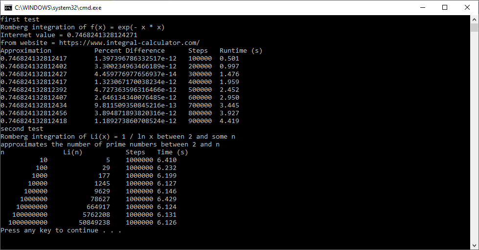
We use two numerical analysis algorithms and two artificial intelligent methods. The first two techniques are from the excellent tome “A Numerical Library in C for Scientists and Engineers” by H.T. Lau, PhD. One does not utilize any derivatives and the other requires first partial derivatives. My homegrown algorithms are my implementation of the particle swarm optimization and an evolutionary hill-climber. The output from my C# application is below:
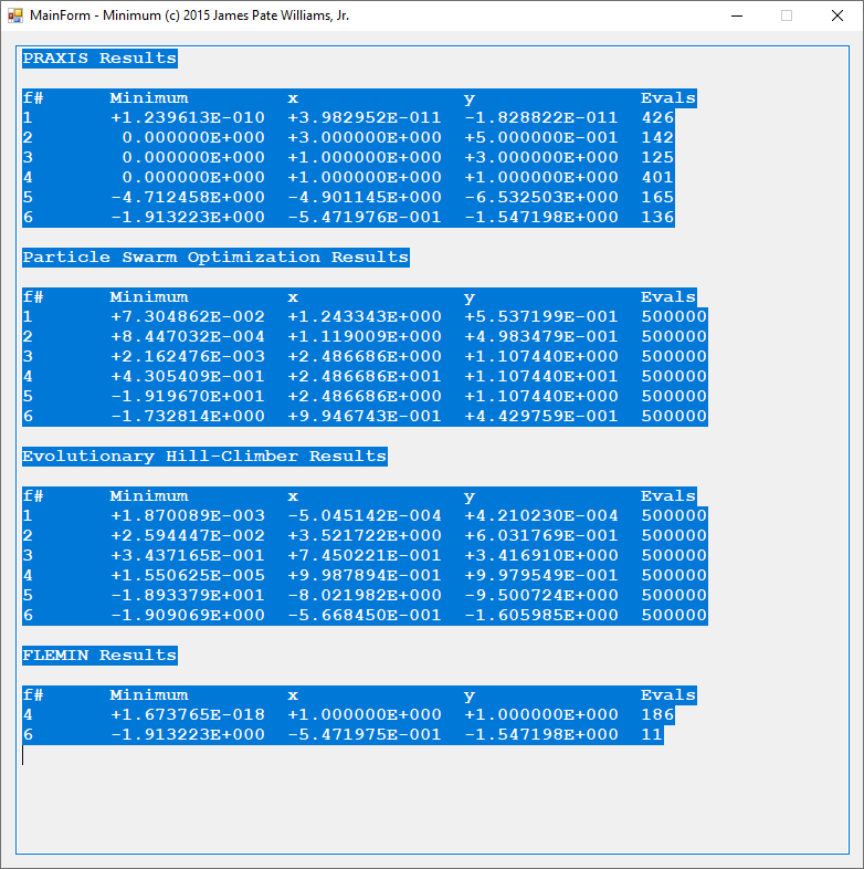
The two numerical algorithms PRAXIS and FLEMIN perform fairly well and do not require that many function evaluations which is better metric than wall-clock time.
See the excellent webpage: https://en.wikipedia.org/wiki/Test_functions_for_optimization
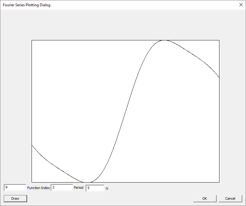
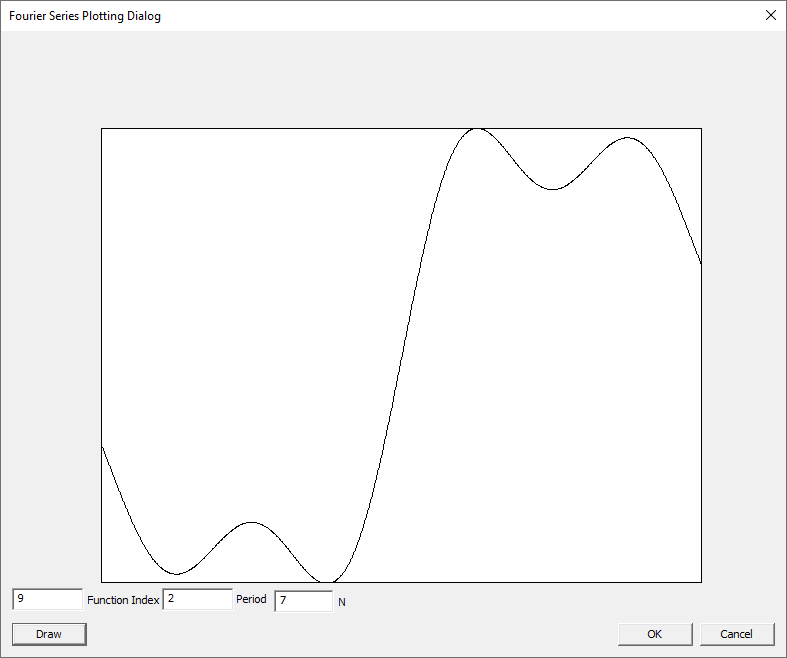
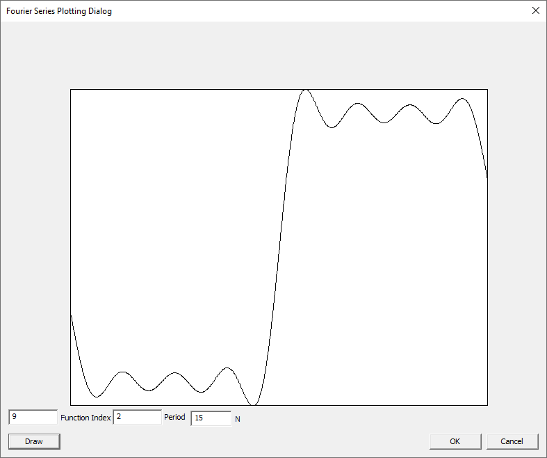
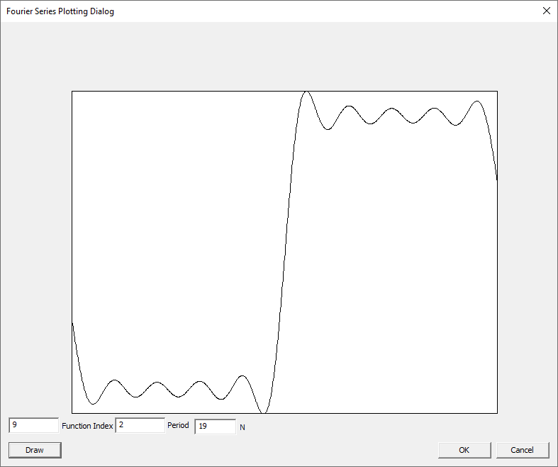
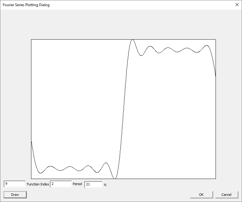
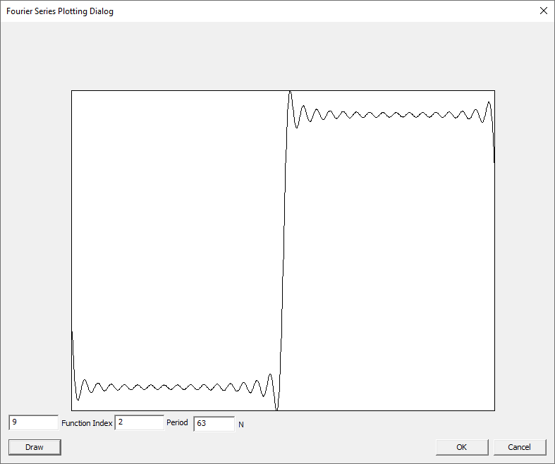
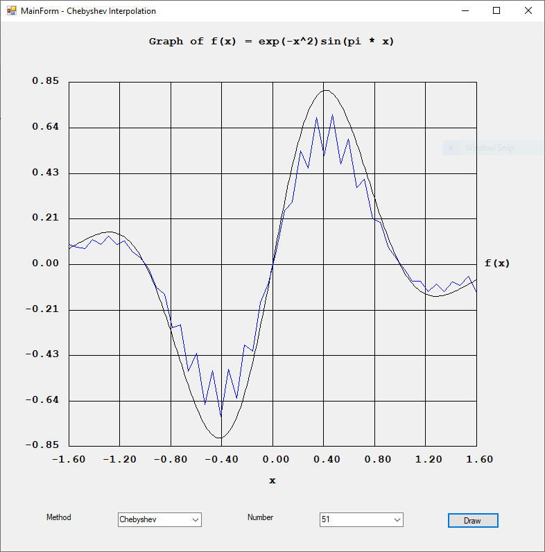
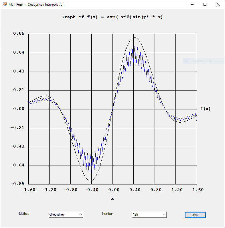
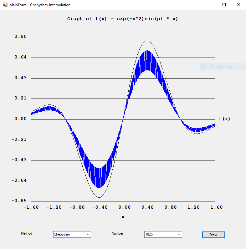
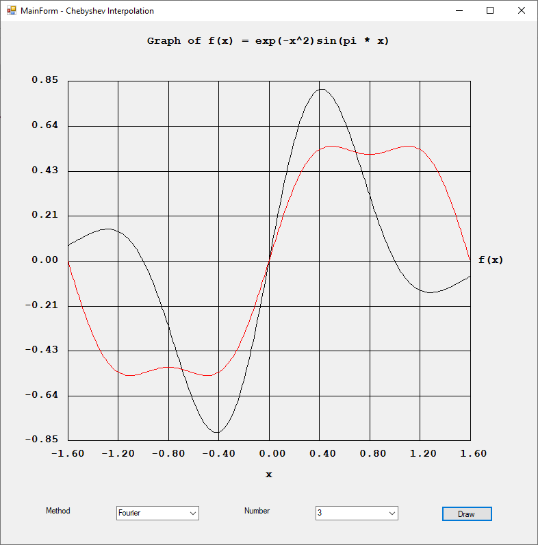
The Gibb’s overshoot phenomenon is very well defined by the Fourier series expansion of the Heaviside step function. The following images were produced by a new C/C++ Win32 application that I created in the period February 10, 2023, to February 14, 2023.
The code was adapted from “Fourier Series and Boundary Value Problems” by Ruel V. Churchill and James Ward Brown. The integration algorithm was translated from C source code found in the tome “A Numerical Library in C for Scientists and Engineers” by H.T. Lau, PhD pages 299-303.