/*
Author: Pate Williams (c) January 22, 1995
The following program is a translation of the FORTRAN
subprogram found in Elementary Numerical Analysis by
S. D. Conte and Carl de Boor pages 343-344. The program
uses Romberg extrapolation to find the integral of a
function.
*/
#include "stdafx.h"
#include <math.h>
#include <stdlib.h>
#include <time.h>
#include <stdio.h>
typedef long double real;
real t[10][10];
real f(real x)
{
return(expl(-x * x));
}
real Li(real x)
{
return(1.0 / logl(x));
}
real romberg(
real a, real b, int start, int row,
real(*f)(real))
{
int i, k, m;
real h, ratio, sum;
m = start;
h = (b - a) / m;
sum = 0.5 * (f(a) + f(b));
if (m > 1)
for (i = 1; i < m; i++)
sum += f(a + i * h);
t[1][1] = h * sum;
if (row < 2) return(t[1][1]);
for (k = 2; k <= row; k++)
{
h = 0.5 * h;
m *= 2;
sum = 0.0;
for (i = 1; i <= m; i += 2)
sum += f(a + h * i);
t[k][1] = 0.5 * t[k - 1][1] + sum * h;
for (i = 1; i < k; i++)
{
t[k - 1][i] = t[k][i] - t[k - 1][i];
t[k][i + 1] = t[k][i] - t[k - 1][i] /
(powl(4.0, (real)i) - 1.0);
}
}
if (row < 3) return(t[2][2]);
for (k = 1; k <= row - 2; k++)
for (i = 1; i <= k; i++)
{
if (t[k + 1][i] == 0.0)
ratio = 0.0;
else
ratio = t[k][i] / t[k + 1][i];
t[k][i] = ratio;
}
return(t[row][row - 1]);
}
int main(void)
{
long double experimental = 0.7468241328124271;
int row = 8;
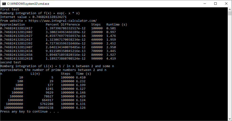
printf("first test\n");
printf("Romberg integration of f(x) = exp(- x * x)\n");
printf("Internet value = 0.7468241328124271\n");
printf("from website = https://www.integral-calculator.com/\n");
printf("Approximation\t\tPercent Difference\tSteps\tRuntime (s)\n");
for (long steps = 100000; steps <= 900000; steps += 100000)
{
clock_t start = clock();
long double trial = romberg(0.0, 1.0, steps, row, f);
clock_t endTm = clock();
long double runtime = ((long double)endTm - start) /
CLOCKS_PER_SEC;
long double pd = 100.0 * fabsl(experimental - trial) /
(0.5 *(experimental + trial));
printf("%16.15lf\t%16.15le\t%6d\t%4.3lf\n",
trial, pd, steps, runtime);
}
printf("second test\n");
printf("Romberg integration of Li(x) = 1 / ln x between 2 and some n\n");
printf("approximates the number of prime numbers between 2 and n\n");
printf("n\t\tLi(n)\t\tSteps\tTime (s)\n");
for (long n = 10; n <= 1000000000; n *= 10)
{
long steps = 1000000;
clock_t start = clock();
long double trial = romberg(2.0, n, steps, row, Li);
clock_t endTm = clock();
long double runtime = ((long double)endTm - start) /
CLOCKS_PER_SEC;
printf("%12ld\t%12.0lf\t%7ld\t%4.3lf\n",
n, trial, steps, runtime);
}
return(0);
}
/*
Author:  Pate Williams (c) January 20, 1995
The following is a translation of the Pascal program
sieve found in Pascalgorithms by Edwin D. Reilly and
Francis D. Federighi page 652. This program uses sets
to represent the sieve (see C Programming Language An
Applied Perspective by Lawrence Miller and Alec Qui-
lici pages 160 - 162).
*/
#include "stdafx.h"
#include <math.h>
#include <stdio.h>
#include <time.h>

#define _WORD_SIZE 32
#define _VECT_SIZE 31250000
#define SET_MIN    0
#define SET_MAX    1000000000

typedef long LONG;
typedef long SET[_VECT_SIZE];
typedef LONG ELEMENT;

SET set;

static LONG get_bit_pos(LONG *long_ptr, LONG *bit_ptr,
	ELEMENT element)
{
	*long_ptr = element / _WORD_SIZE;
	*bit_ptr = element % _WORD_SIZE;
	return(element >= SET_MIN && element <= SET_MAX);
}

static void set_bit(ELEMENT element, LONG inset)
{
	LONG bit, word;

	if (get_bit_pos(&word, &bit, element))
		inset ? set[word] |= (01 << bit) :
		set[word] &= ~(01 << bit);
}

static int get_bit(ELEMENT element)
{
	LONG bit, word;

	return(get_bit_pos(&word, &bit, element) ?
		(set[word] >> bit) & 01 : 0);
}

void set_Add(ELEMENT element)
{
	set_bit(element, 1);
}

void set_Del(ELEMENT element)
{
	set_bit(element, 0);
}

int set_Mem(ELEMENT element)
{
	return get_bit(element);
}

void primes(LONG n)
{
	LONG c, i, inc, k;
	double x;

	clock_t now = clock();
	set_Add(2);
	for (i = 3; i <= n; i++)
		if ((i + 1) % 2 == 0)
			set_Add(i);
		else
			set_Del(i);
	c = 3;
	do
	{
		i = c * c;
		inc = c + c;
		while (i <= n)
		{
			set_Del(i);
			i = i + inc;
		}
		c += 2;
		while (set_Mem(c) == 0) c += 1;
	} while (c * c <= n);
	k = 0;
	for (i = 2; i <= n; i++)
		if (set_Mem(i) == 1) k++;
	x = n / log(n) - 5.0;
	x = x + exp(1.0 + 0.15 * log(n) * sqrt(log(n)));
	clock_t later = clock();
	double runtime = (double)(later - now) / CLOCKS_PER_SEC;
	printf("%10ld\t%10ld\t%10.0lf\t%6.4lf\n",
		n, k, x, runtime);
}

int main(void)
{
	LONG n = 10L;

	printf("--------------------------------------------------------\n");
	printf("n\t\tprimes\t\ttheory\t\ttime (s)\n");
	printf("--------------------------------------------------------\n");
	do
	{
		primes(n);
		clock_t later = clock();
		n = 10L * n;
	} while (n < 1000000000);
	printf("--------------------------------------------------------\n");
	return(0);
}
/*
Author: Pate Williams (c) January 22, 1995
The following program is a translation of the FORTRAN
subprogram found in Elementary Numerical Analysis by
S. D. Conte and Carl de Boor pages 343-344. The program
uses Romberg extrapolation to find the integral of a
function.
*/
#include "stdafx.h"
#include <math.h>
#include <stdlib.h>
#include <time.h>
#include <stdio.h>
typedef long double real;
real t[10][10];
real f(real x)
{
return(expl(-x * x));
}
real romberg(real a, real b, int start, int row)
{
int i, k, m;
real h, ratio, sum;
m = start;
h = (b - a) / m;
sum = 0.5 * (f(a) + f(b));
if (m > 1)
for (i = 1; i < m; i++)
sum += f(a + i * h);
t[1][1] = h * sum;
if (row < 2) return(t[1][1]);
for (k = 2; k <= row; k++)
{
h = 0.5 * h;
m *= 2;
sum = 0.0;
for (i = 1; i <= m; i += 2)
sum += f(a + h * i);
t[k][1] = 0.5 * t[k - 1][1] + sum * h;
for (i = 1; i < k; i++)
{
t[k - 1][i] = t[k][i] - t[k - 1][i];
t[k][i + 1] = t[k][i] - t[k - 1][i] /
(powl(4.0, (real)i) - 1.0);
}
}
if (row < 3) return(t[2][2]);
for (k = 1; k <= row - 2; k++)
for (i = 1; i <= k; i++)
{
if (t[k + 1][i] == 0.0)
ratio = 0.0;
else
ratio = t[k][i] / t[k + 1][i];
t[k][i] = ratio;
}
return(t[row][row - 1]);
}
int main(void)
{
long double experimental = 0.7468241328124271;
int row = 8;
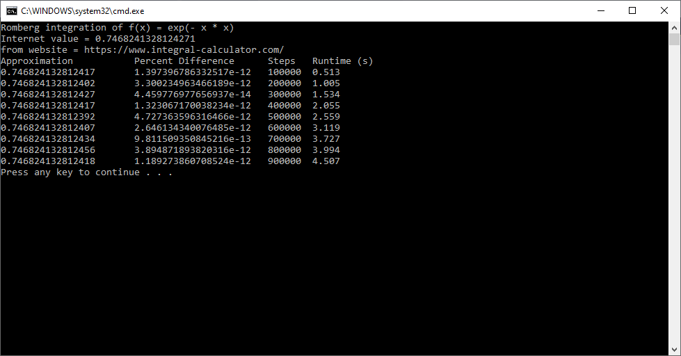
printf("Romberg integration of f(x) = exp(- x * x)\n");
printf("Internet value = 0.7468241328124271\n");
printf("from website = https://www.integral-calculator.com/\n");
printf("Approximation\t\tPercent Difference\tSteps\tRuntime (s)\n");
for (long steps = 100000; steps <= 900000; steps += 100000)
{
clock_t start = clock();
long double trial = romberg(0.0, 1.0, steps, row);
clock_t endTm = clock();
long double runtime = ((long double)endTm - start) /
CLOCKS_PER_SEC;
long double pd = 100.0 * fabsl(experimental - trial) /
(0.5 *(experimental + trial));
printf("%16.15lf\t%16.15le\t%6d\t%4.3lf\n",
trial, pd, steps, runtime);
}
return(0);
}
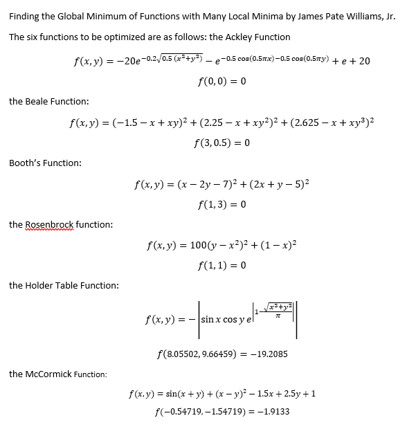
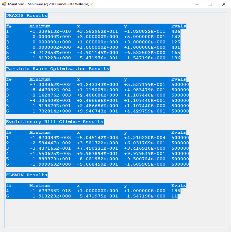
We use two numerical analysis algorithms and two artificial intelligent methods. The first two techniques are from the excellent tome “A Numerical Library in C for Scientists and Engineers” by H.T. Lau, PhD. One does not utilize any derivatives and the other requires first partial derivatives. My homegrown algorithms are my implementation of the particle swarm optimization and an evolutionary hill-climber. The output from my C# application is below:
The two numerical algorithms PRAXIS and FLEMIN perform fairly well and do not require that many function evaluations which is better metric than wall-clock time.
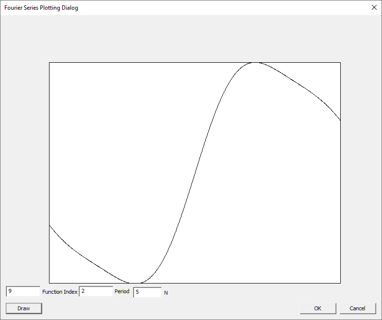
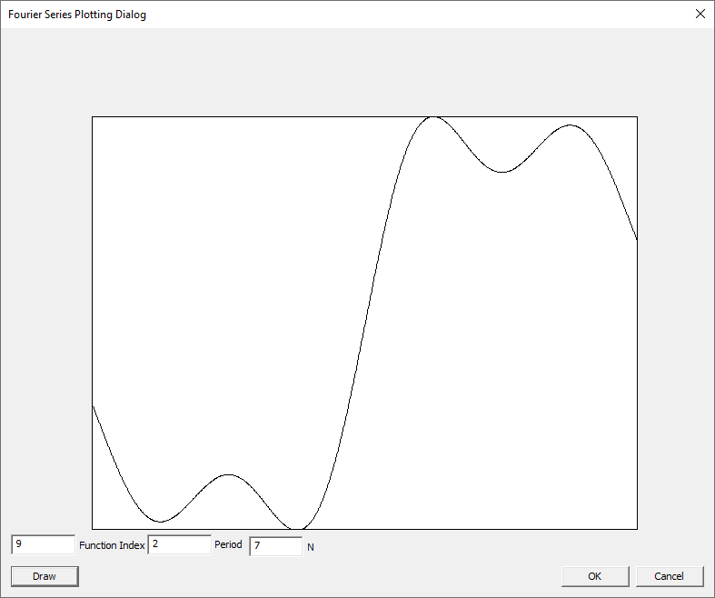
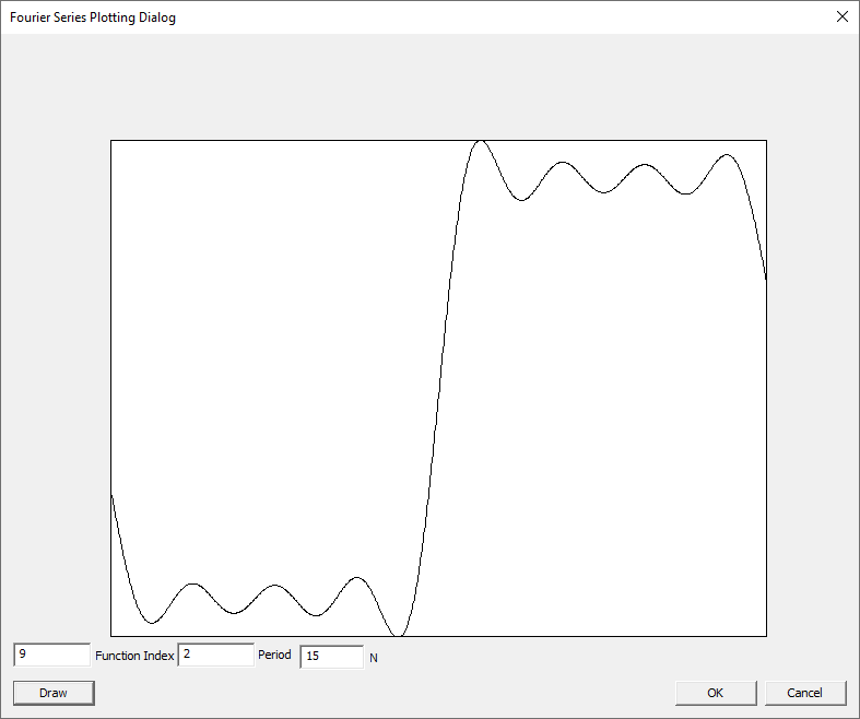
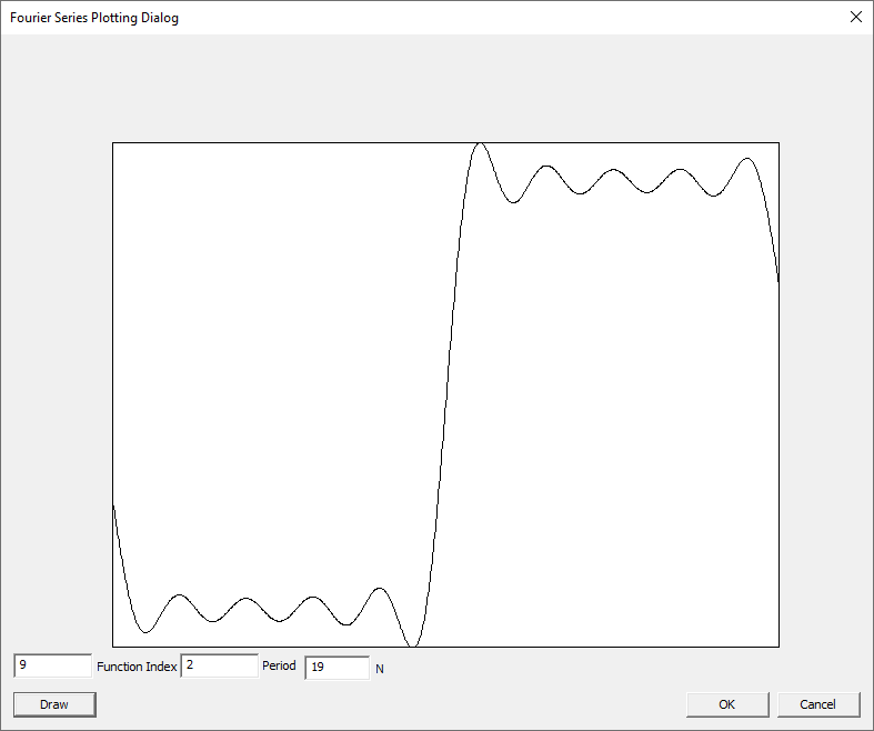
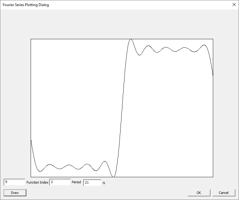
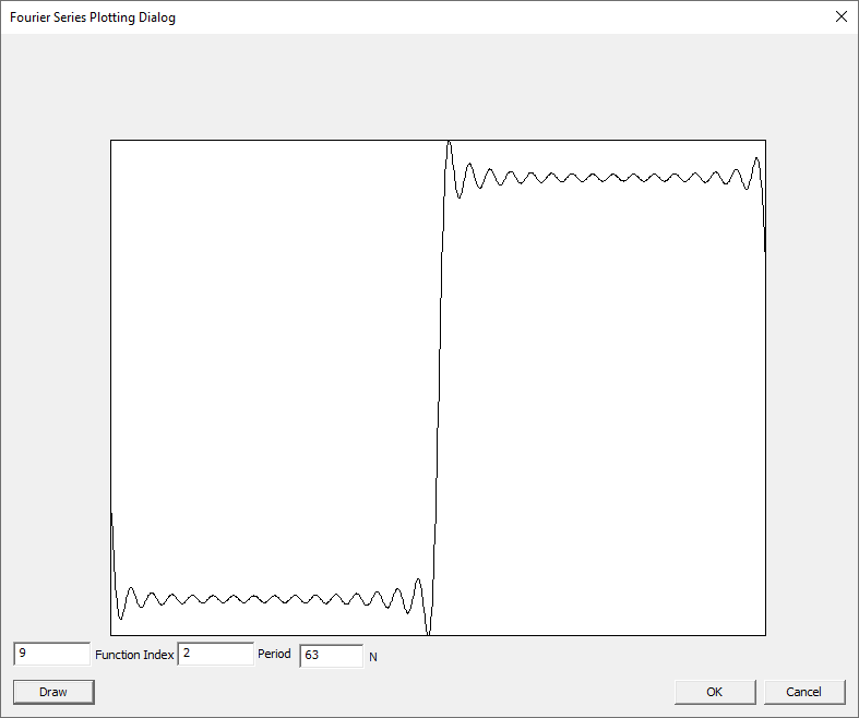
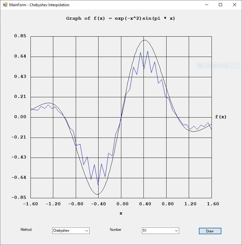
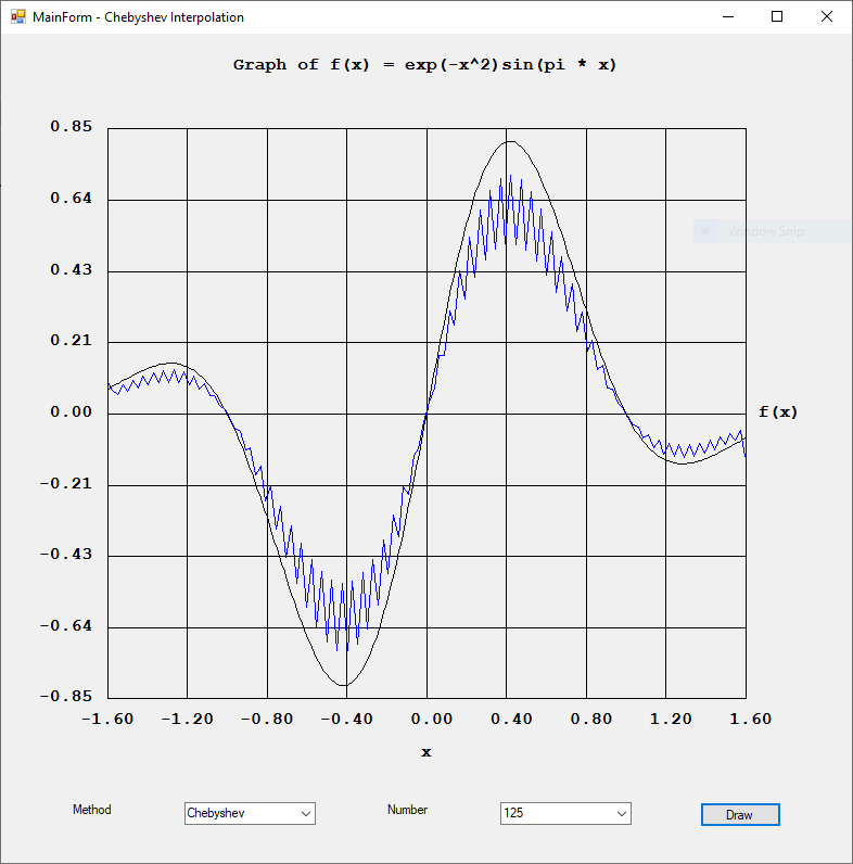
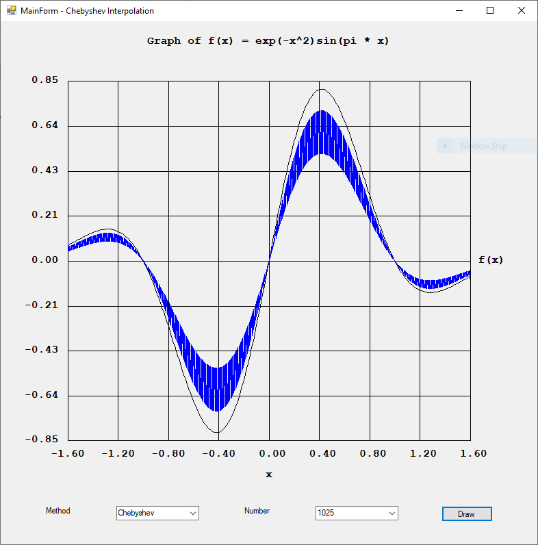
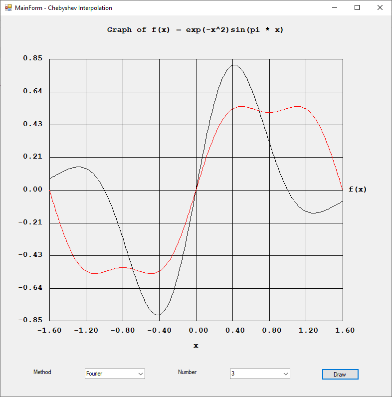
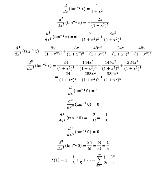
The Gibb’s overshoot phenomenon is very well defined by the Fourier series expansion of the Heaviside step function. The following images were produced by a new C/C++ Win32 application that I created in the period February 10, 2023, to February 14, 2023.
The code was adapted from “Fourier Series and Boundary Value Problems” by Ruel V. Churchill and James Ward Brown. The integration algorithm was translated from C source code found in the tome “A Numerical Library in C for Scientists and Engineers” by H.T. Lau, PhD pages 299-303.
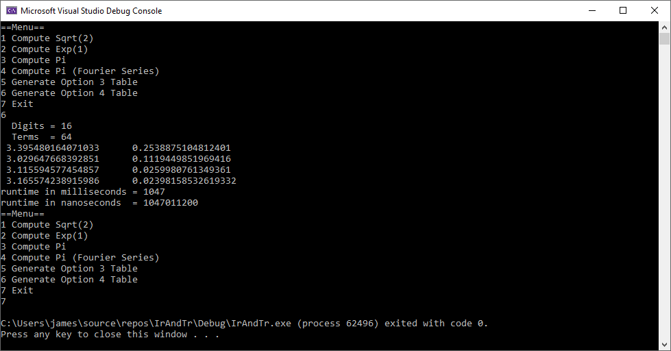
I use a very slowly converging infinite series and Fourier series to compute Pi.
// https://en.wikipedia.org/wiki/Rexx#NUMERIC\
// Translated from Rexx code
// by James Pate Williams, Jr.
// Added a lot of functionality
// Copyrighted February 7 - 10, 2023

#include "FourierSeries.h"
#include <stdlib.h>
#include <iomanip>
#include <iostream>
#include <chrono>
using namespace std;
typedef chrono::high_resolution_clock Clock;

void Option3(int digits, int N)
{
    long double i = 0;
    long double sgn = 1;
    long double sum = 0;
    long double pi0 = Pi;
    long double pi1 = 0.0;

    while (i <= N)
    {
        sum += sgn / (2.0 * i + 1);
        sgn *= -1;
        i = i + 1.0;
    }

    pi1 = 4.0 * sum;
    cout << setw(static_cast<std::streamsize>((int)digits) + 2);
    cout << setprecision(digits) << pi1 << '\t';
    cout << setprecision(digits) << (fabsl(pi0 - pi1)) << endl;
}

void Option4(int digits, int N)
{
    long double* a = new long double[N + 1];
    long double* b = new long double[N + 1];
    memset(a, 0, (N + 1) * sizeof(long double));
    memset(b, 0, (N + 1) * sizeof(long double));
    FourierSeries::CreateCosSeries(N, a);
    FourierSeries::CreateSinSeries(N, b);
    long double pi = 4.0 * FourierSeries::Series(N, 1.0, a, b);
    cout << setw(static_cast<std::streamsize>((int)digits) + 2);
    cout << setprecision(digits) << pi << '\t';
    cout << setprecision(digits) << (fabsl(pi - Pi)) << endl;
    delete[] a;
    delete[] b;
}

int main()
{
    int choice, digits, N = 0, N1 = 0;

    while (1)
    {
        cout << "==Menu==" << endl;
        cout << "1 Compute Sqrt(2)" << endl;
        cout << "2 Compute Exp(1)" << endl;
        cout << "3 Compute Pi" << endl;
        cout << "4 Compute Pi (Fourier Series)" << endl;
        cout << "5 Generate Option 3 Table" << endl;
        cout << "6 Generate Option 4 Table" << endl;
        cout << "7 Exit" << endl;
        cin >> choice;
        if (choice == 7)
            break;
        cout << "  Digits = ";
        cin >> digits;
        if (choice >= 3)
        {
            cout << "  Terms  = ";
            cin >> N;
            N1 = N + 1;
        }
        auto start_time = Clock::now();
        if (choice == 1)
        {
            long double n = 2;
            long double r = 1;
            while (1)
            {
                long double rr = (n / r + r) / 2;
                if (rr == r)
                    break;
                r = rr;
            }

            cout << setprecision(digits) << r << endl;
        }
        else if (choice == 2)
        {
            long double e = 2.5;
            long double f = 0.5;
            long double n = 3;
            do
            {
                f /= n;
                long double ee = e + f;
                if (ee == e)
                    break;
                e = ee;
                n += 1;
            } while (1);

            cout << setprecision(digits) << e << endl;
        }
        else if (choice == 3)
            Option3(digits, N);
        else if (choice == 4)
            Option4(digits, N);
        else if (choice == 5)
        {
            for (int n = 8; n <= N; n *= 2)
                Option3(digits, n);
        }
        else if (choice == 6)
        {
            for (int n = 8; n <= N; n *= 2)
                Option4(digits, n);
        }
        auto end_time = Clock::now();
        cout << "runtime in milliseconds = ";
        cout << std::chrono::duration_cast<std::chrono::milliseconds>
            (end_time - start_time).count();
        cout << endl;
        cout << "runtime in nanoseconds  = ";
        cout << std::chrono::duration_cast<std::chrono::nanoseconds>
            (end_time - start_time).count();
        cout << endl;
    }

    return 0;
}
#pragma once

const long double c = 2.0e9;
const long double Pi = 3.1415926535897932384626433832795;

class FourierSeries
{
private:
	static long double f(long double x);
	static long double cosTermFunction(int n, long double x);
	static long double sinTermFunction(int n, long double x);
public:
	static void CreateCosSeries(int N, long double a[]);
	static void CreateSinSeries(int N, long double b[]);
	static long double Series(int N, long double x,
		long double a[], long double b[]);
};
#include <math.h>
#include "FourierSeries.h"
#include "Integral.h"

long double FourierSeries::f(long double x)
{
    return atanl(x);
}

long double FourierSeries::cosTermFunction(int n, long double x)
{
    return cosl(n * x * Pi / c) * f(x);
}

long double FourierSeries::sinTermFunction(int n, long double x)
{
    return sinl(n * x * Pi / c) * f(x);
}

void FourierSeries::CreateCosSeries(int N, long double a[])
{
    long double e[7] = { 0 };

    e[1] = e[2] = 1.0e-12;

    for (int n = 0; n <= N; n++)
        a[n] = Integral::integral(
            n, -c, c, cosTermFunction, e, 1, 1) / c;
}

void FourierSeries::CreateSinSeries(int N, long double b[])
{
    long double e[7] = { 0 };

    e[1] = e[2] = 1.0e-12;

    for (int n = 1; n <= N; n++)
        b[n] = Integral::integral(
            n, -c, c, sinTermFunction, e, 1, 1) / c;
}

long double FourierSeries::Series(int N, long double x,
    long double a[], long double b[])
{
    long double sum = 0.0;

    for (int n = 1; n <= N; n++)
        sum += a[n] * cosl(2.0 * n * x) + b[n] * sinl(2.0 * n * x);

    return a[0] / 2.0 + sum / 2.0;
}
#pragma once

// Translated from C source code found in the tome
// "A Numerical Library in C for Scientists and
// Engineers" by H.T. Lau, PhD

class Integral
{
private:
	static long double integralqad(
		int n,
		int transf, long double (*fx)(int, long double), long double e[],
		long double* x0, long double* x1, long double* x2, long double* f0, long double* f1,
		long double* f2, long double re, long double ae, long double b1);
	static void integralint(
		int n,
		int transf, long double (*fx)(int, long double), long double e[],
		long double* x0, long double* x1, long double* x2, long double* f0, long double* f1,
		long double* f2, long double* sum, long double re, long double ae, long double b1,
		long double hmin);
public:
	static long double integral(int n, long double a, long double b,
		long double (*fx)(int, long double), long double e[],
		int ua, int ub);
};
#include <math.h>
#include "Integral.h"

long double Integral::integral(
	int n,
	long double a, long double b,
	long double (*fx)(int, long double), long double e[],
	int ua, int ub)
{
	long double x0, x1, x2, f0, f1, f2, re, ae, b1 = 0, x;

	re = e[1];
	if (ub)
		ae = e[2] * 180.0 / fabsl(b - a);
	else
		ae = e[2] * 90.0 / fabsl(b - a);
	if (ua) {
		e[3] = e[4] = 0.0;
		x = x0 = a;
		f0 = (*fx)(n, x);
	}
	else {
		x = x0 = a = e[5];
		f0 = e[6];
	}
	e[5] = x = x2 = b;
	e[6] = f2 = (*fx)(n, x);
	e[4] += integralqad(n, 0, fx, e, &x0, &x1, &x2, &f0, &f1, &f2, re, ae, b1);
	if (!ub) {
		if (a < b) {
			b1 = b - 1.0;
			x0 = 1.0;
		}
		else {
			b1 = b + 1.0;
			x0 = -1.0;
		}
		f0 = e[6];
		e[5] = x2 = 0.0;
		e[6] = f2 = 0.0;
		ae = e[2] * 90.0;
		e[4] -= integralqad(n, 1, fx, e, &x0, &x1, &x2, &f0, &f1, &f2, re, ae, b1);
	}
	return e[4];
}

long double Integral::integralqad(
	int n,
	int transf, long double (*fx)(int, long double), long double e[],
	long double* x0, long double* x1, long double* x2, long double* f0, long double* f1,
	long double* f2, long double re, long double ae, long double b1)
{
	/* this function is internally used by INTEGRAL */

	long double sum, hmin, x, z;

	hmin = fabs((*x0) - (*x2)) * re;
	x = (*x1) = ((*x0) + (*x2)) * 0.5;
	if (transf) {
		z = 1.0 / x;
		x = z + b1;
		(*f1) = (*fx)(n, x) * z * z;
	}
	else
		(*f1) = (*fx)(n, x);
	sum = 0.0;
	integralint(n, transf, fx, e, x0, x1, x2, f0, f1, f2, &sum, re, ae, b1, hmin);
	return sum / 180.0;
}

void Integral::integralint(
	int n,
	int transf, long double (*fx)(int, long double), long double e[],
	long double* x0, long double* x1, long double* x2, long double* f0, long double* f1,
	long double* f2, long double* sum, long double re, long double ae, long double b1,
	long double hmin)
{
	/* this function is internally used by INTEGRALQAD of INTEGRAL */

	int anew;
	long double x3, x4, f3, f4, h, x, z, v, t;

	x4 = (*x2);
	(*x2) = (*x1);
	f4 = (*f2);
	(*f2) = (*f1);
	anew = 1;
	while (anew) {
		anew = 0;
		x = (*x1) = ((*x0) + (*x2)) * 0.5;
		if (transf) {
			z = 1.0 / x;
			x = z + b1;
			(*f1) = (*fx)(n, x) * z * z;
		}
		else
			(*f1) = (*fx)(n, x);
		x = x3 = ((*x2) + x4) * 0.5;
		if (transf) {
			z = 1.0 / x;
			x = z + b1;
			f3 = (*fx)(n, x) * z * z;
		}
		else
			f3 = (*fx)(n, x);
		h = x4 - (*x0);
		v = (4.0 * ((*f1) + f3) + 2.0 * (*f2) + (*f0) + f4) * 15.0;
		t = 6.0 * (*f2) - 4.0 * ((*f1) + f3) + (*f0) + f4;
		if (fabsl(t) < fabsl(v) * re + ae)
			(*sum) += (v - t) * h;
		else if (fabsl(h) < hmin)
			e[3] += 1.0;
		else {
			integralint(n, transf, fx, e, x0, x1, x2, f0, f1, f2, sum,
				re, ae, b1, hmin);
			*x2 = x3;
			*f2 = f3;
			anew = 1;
		}
		if (!anew) {
			*x0 = x4;
			*f0 = f4;
		}
	}
}
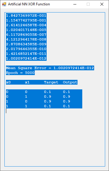
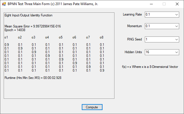
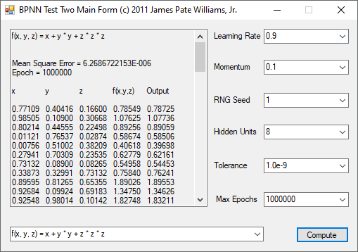
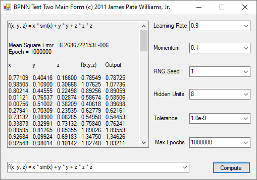
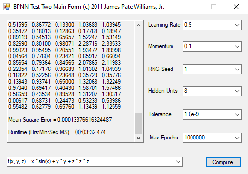
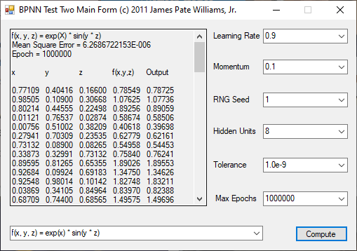
The functions to be calculated are the exclusive or (XOR) function, the eight input and output identity function, and four non-linear three input and one output functions. I used the logistic function that represents 0 as 0.1 and 1 as 0.9. The three input functions use 8 hidden units, a tolerance of 1.0e-9, and maximum number of epochs as 1,000,000. The backpropagation feed-forward neural network algorithm is from Tom M. Mitchell’s classic textbook “Machine Learning” which has a copyright of 1997.
I became interested in attempting to predict temperatures in the state of Georgia way back in the day, i.e., the date was November 1 – 4, 2009. I found a neat website for the temperatures from January 1895 to December 2001. Unfortunately, the website no longer exists online, however, I saved the data to an extinct PC of mine and a USB solid state drive. I used two methods to attempt predictions of the annual temperatures from January 2002 to December 2025. The first algorithm is polynomial least squares curve fitting [1]. The second method is a radial basis function neural network [2] [3] that is trained by an evolutionary hill-climber of my design and implementation [4] [5]. The applications were written in one of my favorite computer programming languages, namely, C# [6].
Methodologies
I created a polynomial least squares dynamic-link library (DLL) using Gaussian elimination with pivoting and an inverse matrix calculation utilizing an upper-triangular matrix [7]. At first the driver application was capable of fitting a 1-degree to 100-degrees polynomial. I found that my algorithm was only valid for a 1-degree to 76-degrees fitting polynomial. I used degrees: 1, 4, 8, 16, 32, 64, and 76.
Predicted Statewide Georgia Annual Average Temperatures in Degrees Fahrenheit
Poly Degree
1
4
8
16
32
64
76
Model
Year
T (F)
T (F)
T (F)
T (F)
T (F)
T (F)
T (F)
Average
2002
64.2
63.1
63.8
63.6
62.4
63.0
62.9
63.3
2003
64.2
63.2
63.6
63.4
64.1
63.7
63.7
63.7
2004
64.2
63.3
63.4
63.4
64.5
63.9
64.0
63.8
2005
64.2
63.3
63.4
63.5
64.2
63.9
64.0
63.8
2006
64.2
63.4
63.4
63.6
63.8
63.7
63.8
63.7
2007
64.2
63.5
63.4
63.7
63.3
63.6
63.6
63.6
2008
64.2
63.6
63.4
63.7
63.0
63.4
63.4
63.5
2009
64.2
63.6
63.4
63.7
62.9
63.3
63.3
63.5
2010
64.1
63.7
63.5
63.7
62.9
63.3
63.2
63.5
2011
64.1
63.8
63.6
63.6
63.1
63.3
63.2
63.5
2012
64.1
63.8
63.7
63.6
63.3
63.4
63.3
63.6
2013
64.1
63.9
63.7
63.6
63.6
63.5
63.5
63.7
2014
64.1
63.9
63.8
63.6
63.9
63.6
63.6
63.8
2015
64.1
64.0
63.9
63.6
64.1
63.8
63.8
63.9
2016
64.1
64.0
63.9
63.6
64.3
63.9
63.9
64.0
2017
64.1
64.1
64.0
63.7
64.4
64.0
64.1
64.1
2018
64.1
64.1
64.1
63.7
64.4
64.1
64.2
64.1
2019
64.1
64.2
64.1
63.9
64.4
64.2
64.2
64.2
2020
64.1
64.2
64.2
64.0
64.3
64.3
64.3
64.2
2021
64.1
64.3
64.2
64.1
64.2
64.3
64.3
64.2
2022
64.1
64.3
64.2
64.2
64.2
64.3
64.3
64.2
2023
64.1
64.3
64.3
64.3
64.1
64.3
64.3
64.2
2024
64.0
64.4
64.3
64.5
64.0
64.3
64.3
64.3
2025
64.0
64.4
64.3
64.6
64.0
64.3
64.3
64.3
The second method was a radial basis function neural network that was trained by an evolutionary hill-climber of my design and implementation. I used 8, 16, 32, 64 basis functions. The population of the hill-climber was 16 and generations 262,144.
Predicted Statewide Georgia Annual Average Temperatures in Degrees Fahrenheit
Basis
8
16
32
64
Model
Year
T (F)
T (F)
T (F)
T (F)
Average
2002
65.4
64.2
65.4
65.2
65.1
2003
65.5
64.2
65.4
65.2
65.1
2004
65.5
64.2
65.5
65.3
65.1
2005
65.5
64.2
65.5
65.3
65.1
2006
65.6
64.2
65.5
65.3
65.2
2007
65.6
64.2
65.6
65.3
65.2
2008
65.6
64.2
65.6
65.4
65.2
2009
65.7
64.2
65.6
65.4
65.2
2010
65.7
64.2
65.6
65.4
65.2
2011
65.7
64.2
65.7
65.4
65.3
2012
65.7
64.2
65.7
65.5
65.3
2013
65.8
64.2
65.7
65.5
65.3
2014
65.8
64.2
65.8
65.5
65.3
2015
65.8
64.3
65.8
65.5
65.4
2016
65.9
64.3
65.8
65.6
65.4
2017
65.9
64.3
65.8
65.6
65.4
2018
65.9
64.3
65.9
65.6
65.4
2019
66.0
64.3
65.9
65.6
65.5
2020
66.0
64.3
65.9
65.7
65.5
2021
66.0
64.3
66.0
65.7
65.5
2022
66.0
64.3
66.0
65.7
65.5
2023
66.1
64.3
66.0
65.7
65.5
2024
66.1
64.3
66.1
65.8
65.6
2025
66.1
64.3
66.1
65.8
65.6
I trust the polynomial fitting results more than the radial basis function neural network values. The polynomial fitting had mean square errors < 1 whereas the radial basis function neural network had mean square errors between 1 and 9. The general trends were increasing temperatures which are in line with the theorized global warming.
References
[1]
H. T. Lau, A Numerical Library in C for Scientists and Engineers, Boca Raton: CRC Press, 1995.
[2]
T. M. Mitchell, Machine Learning, Boston: WCB McGraw-Hill, 1997.
[3]
A. P. Engelbrecht, Computational Intelligence An Introduction, Hoboken: John Wiley and Sons, 2002.
[4]
Z. Michalewicz, Genetic Algorithms + Data Structures = Evolutionary Programs 3rd Edition, Berlin: Springer, 1999.
[5]
D. B. Fogel, Evolutionary Computation Toward a New Philosophy of Machine Intelligence, Piscataway: IEEE Press, 2000.
[6]
C. Petzold, Programming Windows with C#, Redmond: Microsoft Press, 2002.
[7]
S. D. Conte and C. d. Boor, Elementary Numerical An Algorithmic Approach, New York: McGraw-Hill Book Company, 1980.
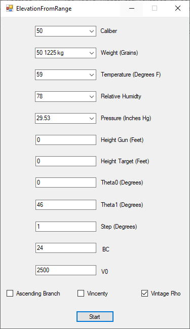
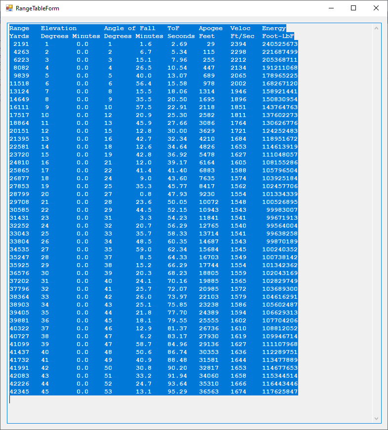
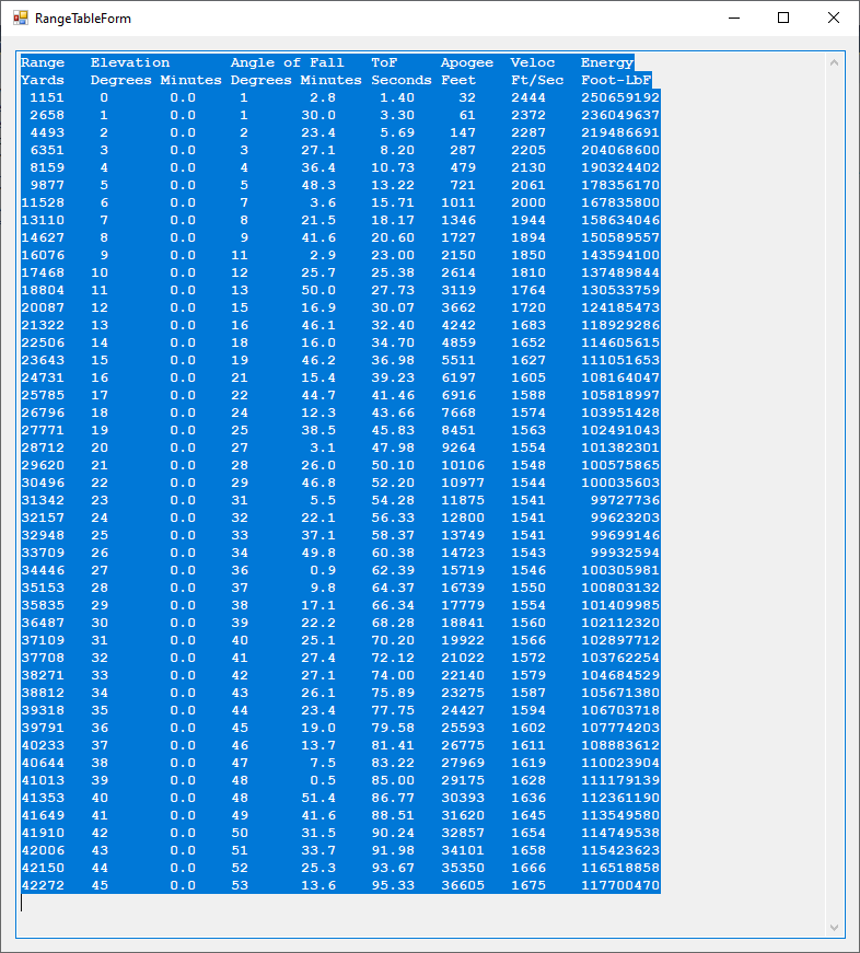
This is another attempt to reproduce the United States Navy’s Ordnance Pamphlet 770: https://eugeneleeslover.com/USN-GUNS-AND-RANGE-TABLES/OP-770-1.html which contains ballistic tables for the battleship USS Iowa (BB-61) artillery (16-inch/50 caliber) and is dated October 1941. My C# Windows desktop application is capable of calculating the elevation from range table which has the columns range in yards, angle of elevation in degrees and minutes, positive angle of fall in degrees and minutes, time of flight in seconds, apogee also called summit in feet, striking velocity in feet per second, and energy in foot pound force. Three corrections can be applied to the trajectory: trunnion height in feet, acceleration of gravity correction, and the curvature of the Earth correction (Vincenty calculation). The first image below is the ballistic settings interface. The second image is the uncorrected table. The third image is the application of a trunnion height of 32 feet. The fourth image is the curvature of the Earth correction. The fifth image is the trunnion height of 32 feet and Vincenty corrections. It is to be noticed that the striking velocity and kinetic energy are the only non-monotonically increasing or decreasing data fields.