using System;

namespace SteadyStateTempCylinder
{
    public class PotPoint : IComparable
    {
        private double x, y, u;

        public double X
        {
            get
            {
                return x;
            }
            set
            {
                x = value;
            }
        }

        public double Y
        {
            get
            {
                return y;
            }
            set
            {
                y = value;
            }
        }

        public double U
        {
            get
            {
                return u;
            }
            set
            {
                u = value;
            }
        }

        public PotPoint(double x, double y, double u)
        {
            this.x = x;
            this.y = y;
            this.u = u;
        }

        public int CompareTo(object obj)
        {
            if (obj == null)
                return 1;

            PotPoint pp = (PotPoint)obj;

            if (u > pp.u)
                return 1;
            else if (u == pp.u)
                return 0;
            else
                return -1;
        }
    }
}
The description of this alphabetic letter game is very facile. Given a word make as many other words as possible using the letters of the given initial word. But first before we enumerate the game solution, we need to refresh the reader’s memory of some elementary mathematics.
The binary number system also known as the base 2 number system is used by computers to perform arithmetic. The digits in the binary number system are 0 and 1. The numbers 0 to 15 in binary using only four binary digits are where ^ is the exponentiation operator (raising a number to a power) are:
0	0000
1	0001	2 ^ 0 = 1
2	0010	2 ^ 1 = 2
3	0011	2 ^ 1 + 2 ^ 0 = 2 + 1 = 3
4	0100	2 ^ 2 = 4
5	0101	2 ^ 2 + 2 ^ 0 = 4 + 1 = 5
6	0110	2 ^ 2 + 2 ^ 1 = 4 + 2 = 6
7	0111	2 ^ 2 + 2 ^ 1 + 2 ^ 0 = 4 + 2 + 1 = 7
8	1000	2 ^ 3 = 8
9	1001	2 ^ 3 + 2 ^ 0 = 8 + 1 = 9
10	1010	2 ^ 3 + 2 ^ 1 = 8 + 2 = 10
11	1011	2 ^ 3 + 2 ^ 1 + 2 ^ 0 = 8 + 2 + 1 = 11
12	1100	2 ^ 3 + 2 ^ 2 = 8 + 4 = 12
13	1101	2 ^ 3 + 2 ^ 2 + 2 ^ 0 = 8 + 4 + 1 = 13
14	1110	2 ^ 3 + 2 ^ 2 + 2 ^ 1 = 8 + 4 + 2 = 14
15	1111	2 ^ 3 + 2 ^ 2 + 2 ^ 1 + 2 ^ 0 = 8 + 4 + 2 + 1 = 15

An algorithm to convert a base 10 (decimal) number to base 2 (binary) number is given below:
Input n a base 10 number
Output b[0], b[1], b[2], … a finite binary string representing the decimal number

Integer i = 0

Do
Integer nmod2 = n mod 2
Integer ndiv2 = n / 2

b[i] = nmod2 + ‘0’
i = i + 1

n = ndiv2

While n > 0

The b[i] will be in reverse order. For example, convert 12 from decimal to using four binary digits:
12 mod 2 = 0
12 div 2 = 6

b[0] = ‘0’

i = 1

n = 6

6 mod 2 = 0
6 div 2 = 3

b[1] = ‘0’

i = 2

n = 3

3 mod 2 = 1
3 div 2 = 1

i = 3

b[2] = ‘1’

n = 1

1 mod 2 = 1
1 div 2 = 0

b[3] = ‘1’

n = 0

So, the reversed binary string of digits is “0011”. And after reversing the string we have 12 is represented by the binary digits “1100”.

Next, we need to define a power set and its binary representation. The index power set of 4 objects which has 2 ^ 4 = 16 entries is specified in the following table:
0	0000
1	0001
2	0010
3	0011
4	0100
5	0101
6	0110
7	0111
8	1000
9	1001
10	1010
11	1011
12	1100
13	1101
14	1110
15	1111
A permutation of the set of three indices is given by the following list:
012, 021, 102, 120, 201, 210

A permutation of n objects is a list of n! = n * (n – 1) * … * 2 * 1. A permutation of 4 objects has a list of 24 – 4-digit indices list since 4! = 4 * 3 * 2 * 1 = 24 has the table:
0123, 0132, 0213, 0231, 0312, 0321,
1023, 1032, 1203, 1230, 1320, 1302,
2013, 2031, 2103, 2130, 2301, 2310,
3012, 3021, 3102, 3120, 3201, 3210

Suppose our word is “lost” then we first find the power set:

1	0001	t
2	0010	s
3	0011	st	ts
4	0100	o
5	0101	ot	to
6	0110	os	so
7	0111	ost	ots	sot	sto	tos	tso
8	1000	l
9	1001	lt	tl
10	1010	ls	sl
11	1011	lst	lts	slt	stl	tsl	tls
12	1100	lo	ol
13	1101	lot	lto	olt	otl	tlo	tol
14	1110	los	lso	slo	sol	osl	ols
15	1111	lost	lots	slot	etc.

Using a dictionary of 152,512 English words my program finds 16 hits for the letters of “lost”:

Dictionary Length: 152512

Word: lost

  0     l
  1     lo
  2     lost
  3     lot
  4     lots
  5     ls
  6     o
  7     s
  8     slot
  9     so
 10     sol
 11     sot
 12     st
 13     t
 14     to
 15     ts

Total letters and/or words 16

Next, we use “tear” as our word:

Dictionary Length: 152512

Word: tear

  0     a
  1     are
  2     art
  3     at
  4     ate
  5     e
  6     ea
  7     ear
  8     eat
  9     era
 10     et
 11     eta
 12     r
 13     rat
 14     rate
 15     re
 16     rt
 17     rte
 18     t
 19     tar
 20     tare
 21     tea
 22     tear
 23     tr

Total letters and/or words 24

Finally, we use the word “company”:

Dictionary Length: 152512

Word: company

  0     a
  1     ac
  2     am
  3     amp
  4     an
  5     any
  6     c
  7     ca
  8     cam
  9     camp
 10     campy
 11     can
 12     canopy
 13     cap
 14     capo
 15     capon
 16     cay
 17     cm
 18     co
 19     com
 20     coma
 21     comp
 22     company
 23     con
 24     cony
 25     cop
 26     copay
 27     copy
 28     coy
 29     cyan
 30     m
 31     ma
 32     mac
 33     man
 34     many
 35     map
 36     may
 37     mayo
 38     mo
 39     moan
 40     mop
 41     mp
 42     my
 43     myna
 44     n
 45     nap
 46     nay
 47     nm
 48     no
 49     o
 50     om
 51     on
 52     op
 53     p
 54     pa
 55     pan
 56     pay
 57     pm
 58     pony
 59     y
 60     ya
 61     yam
 62     yap
 63     yo
 64     yon

Total letters and/or words 65

The C++ program's source code is given below:

// WordToWords.cpp : This file contains the 'main' function. Program execution begins and ends there.
//

#include "pch.h"
#include <algorithm>
#include <fstream>
#include <iomanip>
#include <iostream>
#include <string>
#include <vector>

using namespace std;

vector<string> dictWords;

bool ReadDictionaryFile()
{
    fstream newfile;

    newfile.open("C:\\Users\\james\\source\\repos\\WordToWords\\Dictionary.txt", ios::in);

    if (newfile.is_open()) {
        int index = 0, length = 128;
        char cstr[128];

        while (newfile.getline(cstr, length)) {
            string str;

            str.clear();

            for (int i = 0; i < (int)strlen(cstr); i++)
                str.push_back(cstr[i]);

            dictWords.push_back(str);
        }

        newfile.close();

        sort(dictWords.begin(), dictWords.end());
        return true;
    }

    else
        return false;
}

string ConvertBase2(char cstr[], int n, int len)
{
    int count = 0;
    string str, rev;

    do
    {
        int nMod2 = n % 2;
        int nDiv2 = n / 2;

        str.push_back(nMod2 + '0');
        n = nDiv2;
    } while (n > 0);

    n = str.size();

    for (int i = n; i < len; i++)
        str.push_back('0');

    n = str.size();

    for (int i = n - 1; i >= 0; i--)
        if (str[i] == '1')
            rev.push_back(cstr[i]);

    return rev;
}

vector<string> PowerSet(char cstr[], int len)
{
    vector<int> index;
    vector<string> match;

    for (long ps = 0; ps <= pow(2, len); ps++)
    {
        string str = ConvertBase2(cstr, ps, len);
        int psf = 1;

        for (int i = 2; i <= len; i++)
            psf *= i;

        for (int i = 0; i < psf; i++)
        {
            if (binary_search(dictWords.begin(), dictWords.end(), str))
            {
                if (!binary_search(match.begin(), match.end(), str))
                {
                    match.push_back(str);
                    sort(match.begin(), match.end());
                }
            }

            next_permutation(str.begin(), str.end());
        }

        sort(match.begin(), match.end());
    }

    return match;
}

int main()
{
    bool done = false;
    char cstr[128];
    int len;
    string str;
    vector<int> index;
    vector<string> match;

    if (!ReadDictionaryFile())
        return -1;

    cout << "Dictionary Length: " << dictWords.size() << endl << endl;

    cout << "Word: ";
    cin >> cstr;
    cout << endl;

    len = strlen(cstr);

    if (len != 0)
    {
        vector<string> match = PowerSet(cstr, len);

        for (int i = 0; i < match.size(); i++)
        {
            cout << setprecision(3) << setw(3) << i << "\t";
            cout << match[i] << endl;
        }

        cout << endl;
        cout << "Total letters and/or words " << match.size() << endl;
        cout << endl;
    }
}
Alpha is defined as 0.5 * n. In our case n = 1, 2, 3, 4.
The solutions for the four cases above are graphed using Microsoft Mathematics:
Elliptic Partial Differential Equation for n = 1
Elliptic Partial Differential Equation for n = 2
Elliptic Partial Differential Equation for n = 3
Elliptic Partial Differential Equation for n = 4
The Microsoft Mathematics Application Window is illustrated below:
Microsoft Mathematics Application
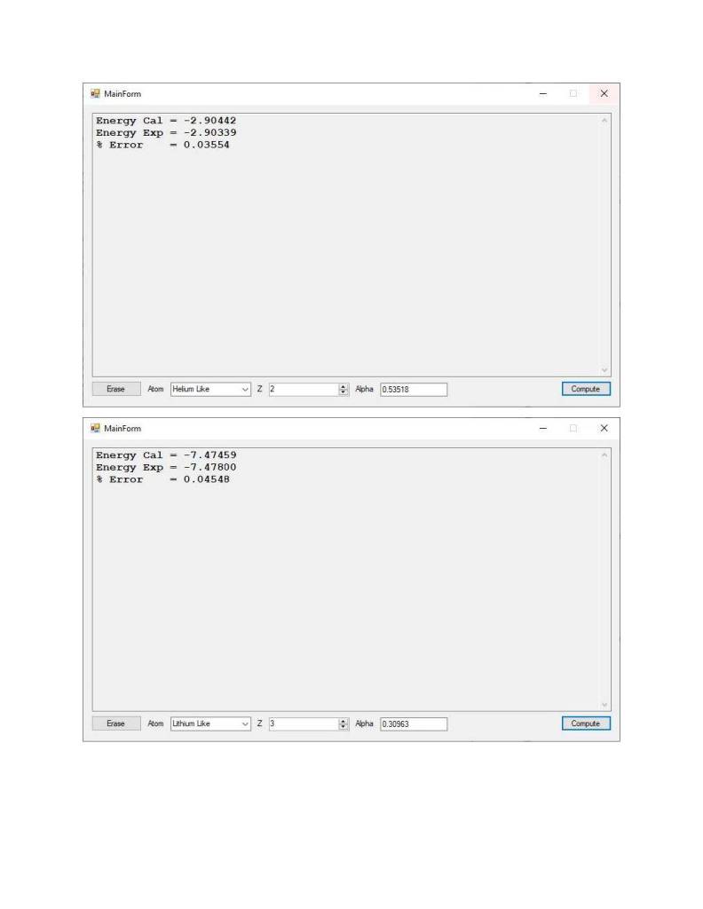
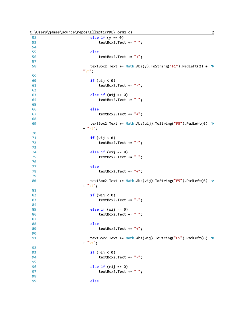
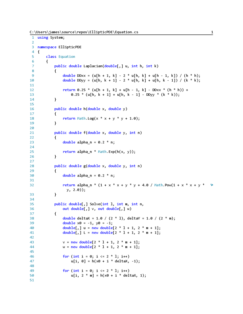
Finite Element Method Elliptic PDF Solver Main Form 1Finite Element Method Elliptic PDF Solver Main Form 2Finite Element Method Elliptic PDF Solver Main Form 3Finite Element Method Elliptic PDF Solver Equation Class 1Finite Element Method Elliptic PDF Solver Equation Class 2
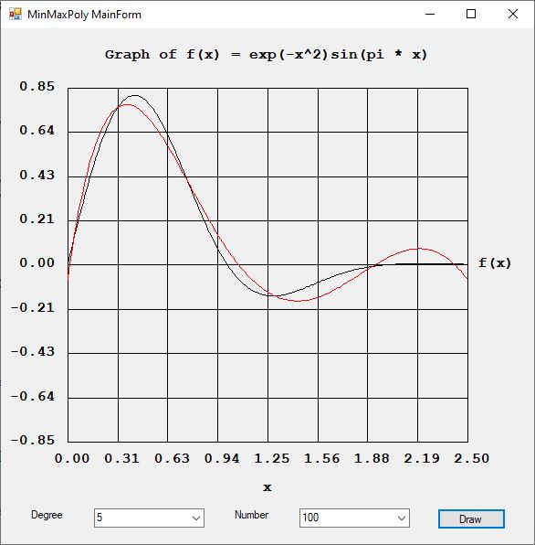
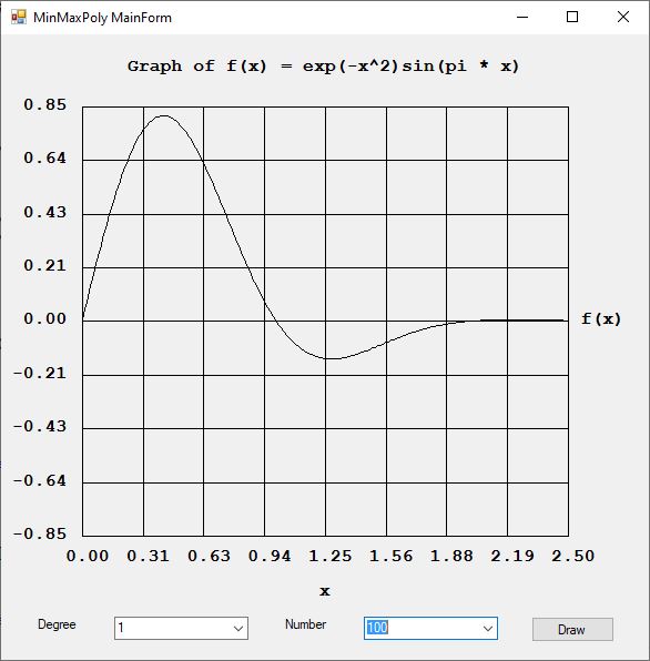
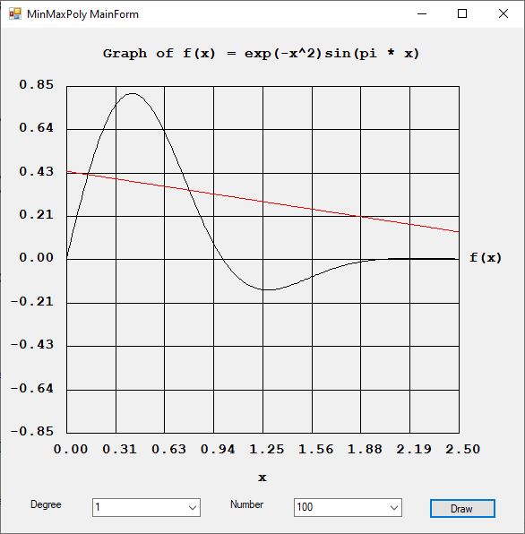
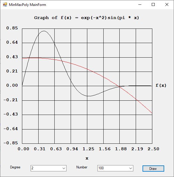
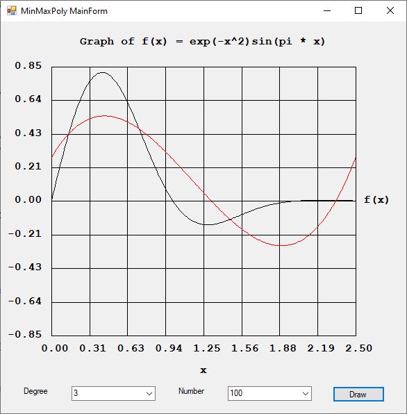
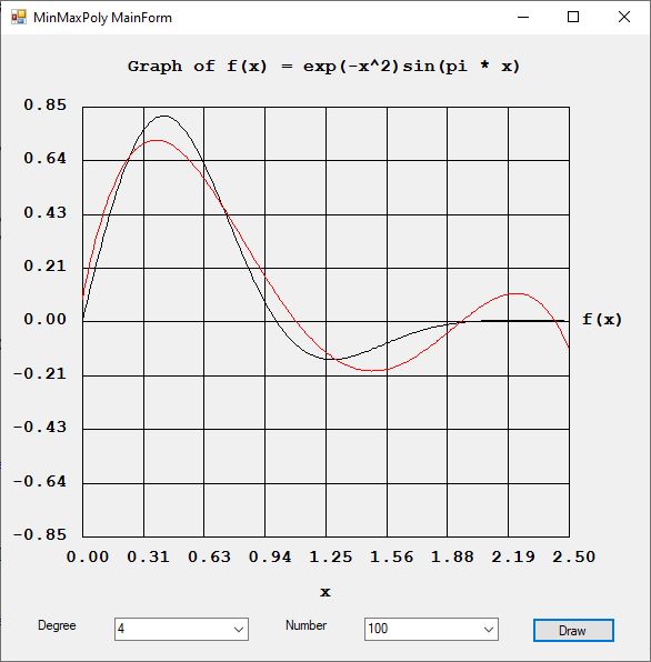
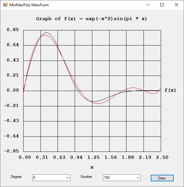
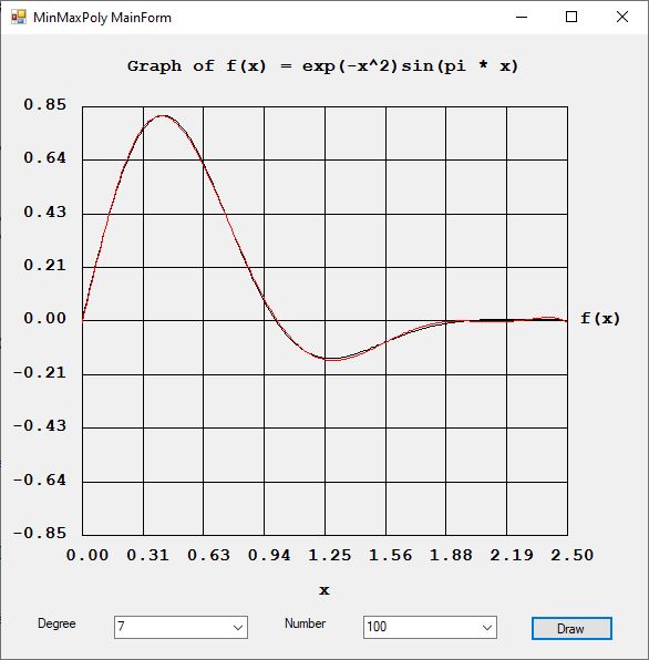
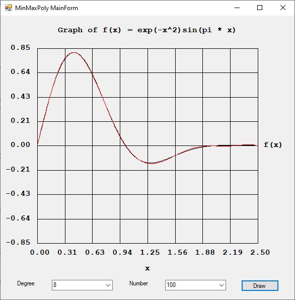
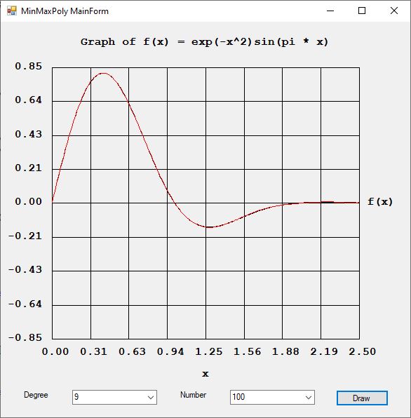
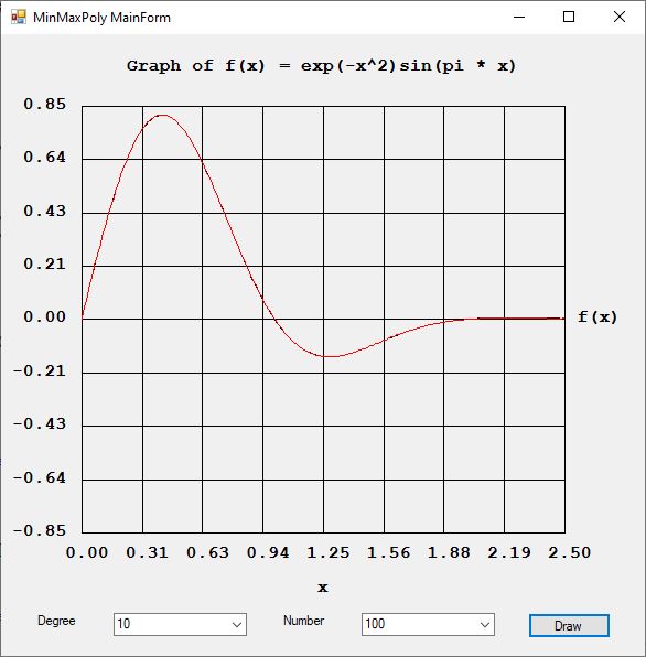
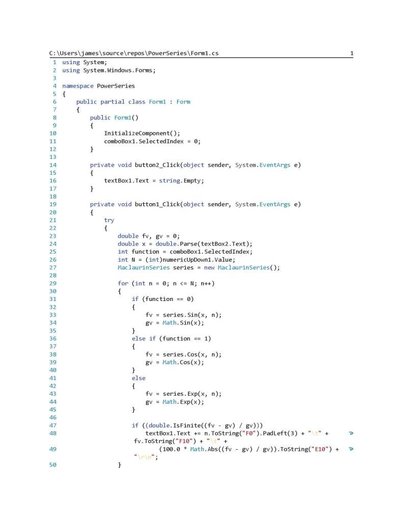
On Sunday, August 28, 2016, 3:57:53 PM I created a C# program to fit a given curve to a polynomial of a specified degree and number of points. Here are ten experiments with a continuous function to be discretely fitted by a polynomial.
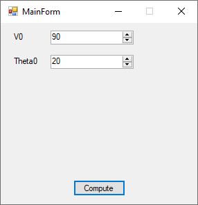
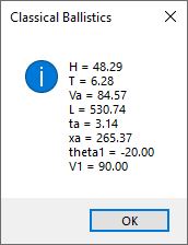
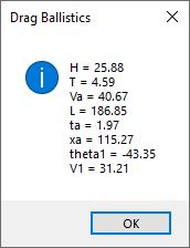
I created a C# application to test the preceding equations against numerical methods of calculating the trajectory of a baseball. The baseball has an initial velocity of 90 miles per hour and an angle of inclination of 20 degrees. The classical model certainly overestimates the trajectory.