I owe the whole staffs of our great and caring local Pathways Center Second Season, WellStar West Georgia Medical Center, and Emory Clark Holder Clinic, a humble and thorough apology. I would like to congratulate Doctor G. Ralston Major II, MD who was pivotal in getting my movement towards physical health started as soon as I was incarcerated for my own good and taken off my feet and diseased legs. I accosted Dr. Major while he was having breakfast one morning with his colleagues at Chick-fil-a. Instead of him getting arrogant and angry he asked me to setup an appointment to see him about my bad hereditary and environmental venous reflux disease. I don’t know if we exchanged business cards at that meeting or not, but he is a true real-life saver. Anyway, to move onward with my story of mental and physical rebirth, I was incarcerated for my own good in Troup County Jail on either Wednesday, May 8, 2019, or Friday, May 10, 2019. After a period of either 35 or 33 days, I was transferred to Pathways Center Second Season of LaGrange, Troup County, Georgia. I fought my internment at the mental health facility tooth and nail because I could not see the whole picture until it became crystal clear to me on Monday, December 23, 2019, or 27 days after my release from being in Troup County Jail again from October 17, 2019, to November 26, 2017, a period of 40 days. I was at Pathways Center Second Season for an astounding 127 days which I am sure is a record number of days that anyone had spent in the facility. Everything came together today with my appointment with Dr. G. Ralston Major II, MD at 2:00 PM this afternoon of Monday, December 23, 2019. Afterwards I finally got around to carefully studying my WellStar MyChart. Anyway, my three to five very costly physical visits to the Emergency Department of WellStar West Georgia Medical Center on June 12, June 13, June 25, August 1, and September 6, 2019, were not in vein (no misspelling pun intended). Notice I was in Pathways Center Second Season and not in the Troup County Jail during the dates of my emergency department treatment. I misbehaved like a potty mouthed adolescent when I was physically in the WellStar West Georgia Medical Center. I was treated with great respect and a very firm hand by the staff of the Emergency Department WellStar West Georgia Medical Center. I would like to give a tremendous shoutout to the following prominent female nursing employee of Pathways Center Second Season, Merry B. I could name a good number of other male and female employees of Pathways Center Second Season and the Troup County Jail, but I will let them reside behind a cloak of anonymity. I have an appointment with Dr. G. Ralston Major II, MD on Thursday, January 30, 2020 for a noninvasive venous reflux vein mapping. I hope to make that appointment, but I must go before state court on Monday, January 27, 2020 for my stupid misbehavior of May 8 or May 10, 2019. I guess I should have known better how to act in public!
Thanks,
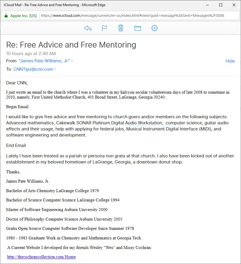
James Pate Williams, Jr.
Bachelor of Arts Chemistry LaGrange College 1979
Bachelor of Science Computer Science LaGrange College 1994
Master of Software Engineering Auburn University 2000
Doctor of Philosophy Computer Science Auburn University 2005
Gratis Open-Source Computer Software Developer Since Summer 1978
1980 – 1983 Graduate Work in Chemistry and Mathematics at Georgia Tech
A Current Website I developed for my friends Wesley “Wes” and Missy Cochran:
http://thecochrancollection.com/Home