Category: C++ Computer Applications
Blog Entry (c) Wednesday, December 18, 2024, Curve Fitting Using Orthogonal Polynomials by James Pate Williams, Jr.
Blog Entry © Saturday, November 30, 2024, by James Pate Williams, Jr. Partial Solution of the Schrödinger Equation for Hydrogen in Parabolic Coordinates
Blog Entry (c) Thursday, November 21, 2024, by James Pate Williams, Jr. Comparison of Homegrown Fifth Order Runge-Kutta Method Versus a Limited Number of Predictor-Corrector Algorithm
The first table is based on Conte-de Boor Fourth Runge-Kutta formulas that I converted to Fifth Order Runge-Kutta. Initial values: V = 2600 feet per second angle of elevation 30 degrees diameter 16 inches coefficient of form 0.61 density ratio 1.00 are from LCDR Ernest Edward Herrmann’s Exterior ballistics, 1935 My results are given first then LCDR Herrmann’s results:
| x | deg | min | sec | time | v | vx | vy | y |
|---|---|---|---|---|---|---|---|---|
| 0 | 30 | 0 | 0 | 0.00 | 2600 | 2252 | 1300 | 0 |
| 563 | 29 | 50 | 45 | 0.25 | 2578 | 2236 | 1283 | 325 |
| 1122 | 29 | 41 | 24 | 0.50 | 2556 | 2221 | 1266 | 646 |
| 1677 | 29 | 31 | 57 | 0.75 | 2535 | 2206 | 1250 | 962 |
| 2229 | 29 | 22 | 25 | 1.00 | 2515 | 2191 | 1233 | 1275 |
| 2776 | 29 | 12 | 47 | 1.25 | 2494 | 2177 | 1217 | 1583 |
| 3321 | 29 | 3 | 4 | 1.50 | 2474 | 2163 | 1201 | 1887 |
| 3861 | 28 | 53 | 15 | 1.75 | 2455 | 2149 | 1186 | 2188 |
| x | deg | min | sec | time | v | vx | vy | y |
|---|---|---|---|---|---|---|---|---|
| 0 | 30 | 0 | 0 | 0.00 | 2600 | 2252 | 1300 | 0 |
| 561 | 29 | 50 | 7 | 0.25 | 2582 | 2259 | 1285 | 323 |
| 1120 | 29 | 41 | 4 | 0.50 | 2564 | 2227 | 1270 | 642 |
| 1675 | 29 | 32 | 2 | 0.75 | 2546 | 2216 | 1255 | 958 |
| 2228 | 29 | 22 | 5 | 1.00 | 2529 | 2204 | 1241 | 1270 |
It is amazing how accurate Herrmann’s results were based on only a couple iterations using the Mayevski seven zone velocity retardation formulas.
Blog Entry © Sunday, November 17, 2024, by James Pate Williams, Jr. Three Methods of Solving the Exterior Ballistics Problem for the Fast Battleship USS Iowa (BB-61) 16-Inch/50 Caliber Rifles
Blog Entry © Saturday, November 16, 2024, by James Pate Williams, Jr., The Microsoft Copilot
Blog Entry © Thursday, November 14, 2024, by James Pate Williams, Jr.
Blog Entry © Wednesday, November 6, 2024, by James Pate Williams, Jr. Particle in a Finite Spherical Three-Dimensional Potential Well
The Bessel functions are from A Numerical Library in C for Scientists and Engineers (c) 1995 by H. T. Lau, PhD.
Blog Entry (c) Wednesday, November 6, 2024, by James Pate Williams, Jr. Small Angular Momentum Quantum Numbers Gaunt Coefficients
// GauntCoefficients.cpp (c) Monday, November 4, 2024
// by James Pate Williams, Jr., BA, BS, MSWE, PhD
// Computes the Gaunt angular momentum coefficients
// Also the Wigner-3j symbols are calculated
// https://en.wikipedia.org/wiki/3-j_symbol
// https://doc.sagemath.org/html/en/reference/functions/sage/functions/wigner.html#
// https://www.geeksforgeeks.org/factorial-large-number/
#include <iostream>
using namespace std;
typedef long double real;
real pi;
// iterative n-factorial function
real Factorial(int n)
{
    real factorial = 1;

    for (int i = 2; i <= n; i++)
        factorial *= i;
    if (n < 0)
        factorial = 0;
    return factorial;
}
real Delta(int lt, int rt)
{
    return lt == rt ? 1.0 : 0.0;
}
real Wigner3j(
    int j1, int j2, int j3,
    int m1, int m2, int m3)
{
    real delta = Delta(m1 + m2 + m3, 0) *
        powl(-1.0, j1 - j2 - m3);
    real fact1 = Factorial(j1 + j2 - j3);
    real fact2 = Factorial(j1 - j2 + j3);
    real fact3 = Factorial(-j1 + j2 + j3);
    real denom = Factorial(j1 + j2 + j3 + 1);
    real numer = delta * sqrt(
        fact1 * fact2 * fact3 / denom);
    real fact4 = Factorial(j1 - m1);
    real fact5 = Factorial(j1 + m1);
    real fact6 = Factorial(j2 - m2);
    real fact7 = Factorial(j2 + m2);
    real fact8 = Factorial(j3 - m3);
    real fact9 = Factorial(j3 + m3);
    real sqrt1 = sqrtl(
        fact4 * fact5 * fact6 * fact7 * fact8 * fact9);
    real sumK = 0;
    int K = (int)fmaxl(0, fmaxl((real)j2 - j3 - m1,
        (real)j1 - j3 + m2));
    int N = (int)fminl((real)j1 + j2 - j3,
        fminl((real)j1 - m1, (real)j2 + m2));
    for (int k = K; k <= N; k++)
    {
        real f0 = Factorial(k);
        real f1 = Factorial(j1 + j2 - j3 - k);
        real f2 = Factorial(j1 - m1 - k);
        real f3 = Factorial(j2 + m2 - k);
        real f4 = Factorial(j3 - j2 + m1 + k);
        real f5 = Factorial(j3 - j1 - m2 + k);
        sumK += powl(-1.0, k) / (f0 * f1 * f2 * f3 * f4 * f5);
    }
    return numer * sqrt1 * sumK;
}
real GauntCoefficient(
    int l1, int l2, int l3, int m1, int m2, int m3)
{
    real factor = sqrtl(
        (2.0 * l1 + 1.0) *
        (2.0 * l2 + 1.0) *
        (2.0 * l3 + 1.0) /
        (4.0 * pi));
    real wigner1 = Wigner3j(l1, l2, l3, 0, 0, 0);
    real wigner2 = Wigner3j(l1, l2, l3, m1, m2, m3);
    return factor * wigner1 * wigner2;
}
int main()
{
    pi = 4.0 * atanl(1.0);
    cout << "Gaunt(1, 0, 1, 1, 0, 0)  = ";
    cout << GauntCoefficient(1, 0, 1, 1, 0, 0);
    cout << endl;
    cout << "Gaunt(1, 0, 1, 1, 0, -1) = ";
    cout << GauntCoefficient(1, 0, 1, 1, 0, -1);
    cout << endl;
    real number = -1.0 / 2.0 / sqrtl(pi);
    cout << "-1.0 / 2.0 / sqrt(pi)    = ";
    cout << number << endl;
    return 0;
}
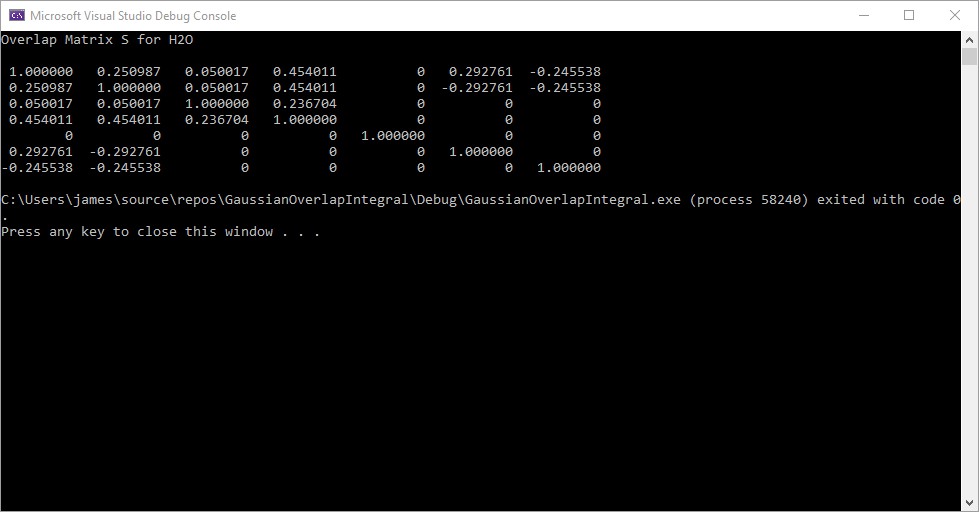
Blog Entry © Friday, November 1, 2024, by James Pate Williams, Jr. Calculation of the Overlap Matrix for the Water Molecule (H2O) Using a Contracted Set of Gaussian Orbitals
Reference: https://content.wolfram.com/sites/19/2012/02/Ho.pdf
I reproduced most of the computations in the MATHMATICA reference. The water molecule is a planar molecule that lies in the YZ-plane.