Category: Numerical Analysis
My Near-Term Agenda by James Pate Williams, Jr. BA, BS, MSwE, PhD
Merry Christmas to all you devout Christians. I am not one of you. I am about to embark on a mission to carefully annotate with open source C# computer code my copy of “Exterior Ballistics, 1935” by Professor Ernest Edward Herrmann of then the United States Naval Academy at Annapolis, Maryland. This book set the standard for naval gunnery in World War II. Of course, our navy and especially our battle-wagons had the largest rifled artillery of any United States service. The 105 mm = 105 mm / 25.4 mm / inch = 4.13 inches, 120 mm / 25.4 mm / inch = 4.72 inches, and 155 mm / 25.4 mm / inch = 6.10 inch of our excellent United States Army and United States Marine Corps (semper fidelis) are puny in comparison to the mighty 8, 10, 12, 14, and finally 16 inch mostly rifled artillery of our incredible navy’s cruisers, dreadnoughts, and battleships of the World War I and World War II era ships. Even a destroyer of the USN Fletcher class had 5-inch (127 mm) / 38 caliber rifled artillery which had a 5 inch * 38 = 190-inch barrel length. Our mightiest naval artillery was, of course, my favorite the mighty 16 inch (406.4 mm) / 50 caliber rifles that had a barrel length of 16 * 50 inches = 800 inches = 66.6 feet!
Thanks,
James Pate Williams, Jr.
Bachelor of Arts Chemistry LaGrange College 1979
Bachelor of Science Computer Science LaGrange College 1994
Master of Software Engineering Auburn University 2000
Doctor of Philosophy Computer Science Auburn University 2005
Gratis Open Source Computer Software Developer Since Summer 1978
1980 – 1983 Graduate Work in Chemistry and Mathematics at Georgia Tech
A Current Website I developed for my friends Wesley “Wes” and Missy Cochran:
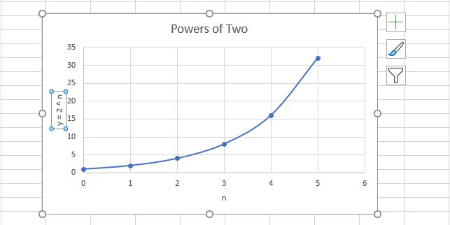
Powers of Two – Excel by James Pate Williams, Jr. BA, BS, MSwE, PhD
First Function in Excel (Assumes that You Have Access to an Office 365 Subscription)
Please attempt the following procedure:
- Type Excel in the Windows 10 Search Box
- Select the Excel App
- Select Blank workbook
- Maximize the Excel Window
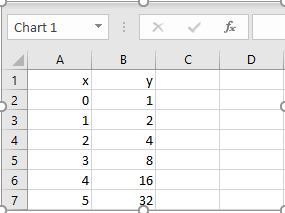
- Type x in Cell A1
- Tab to Cell B1
- Type y in Cell B1
- Type 0 in Cell A2
- Type 1 in Cell B2
- Type 1 in Cell A3
- Type 2 in Cell B3
- Type 2 in Cell A4
- Type 4 in Cell B4
- Type 3 in Cell A5
- Type 8 in Cell B5
- Type 4 in Cell A6
- Type 16 in Cell B6
- Type 5 in Cell A7
- Type 32 in Cell A8
- Highlight Cells A1 and B1
- From the Toolbar Select Alignment and Right Alignment
- Select File Save As
- Select “Documents” and “Powers of Two” as the filename
- Highlight Cells A1 to B7
- Select Insert from Toolbar
- Select Charts Scatter
- Select the Chart
- Select the Big + Sign on the Right
- Label the y-axis “y = 2 ^ n”
- Label the x-axis “n”
- Relabel the Title of the Chart as “Powers of Two”
Note that x is in the finite set { 0, 1, 2, 3, 4, 5 }
Note that y is the function y = 2 ^ x where ^ is the exponentiation operator
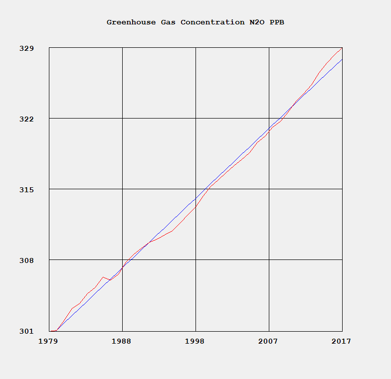
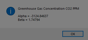
Global Primary Greenhouse Gas Concentrations by James Pate Williams Jr BA, BS, MSwE, PhD
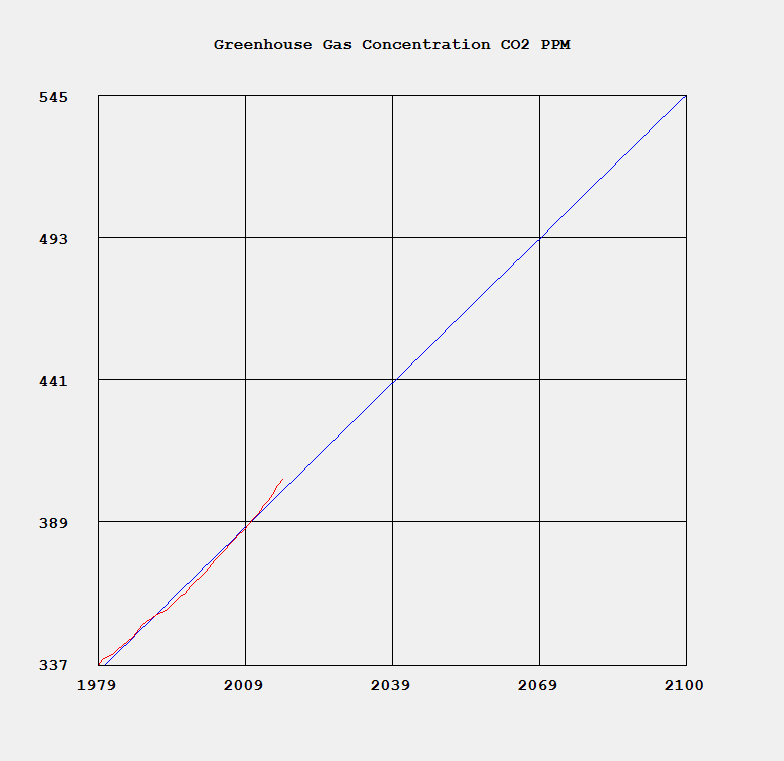
I designed and implemented a C# computer language application to model the global greenhouse gas concentrations data found on the NOAA website:
https://www.esrl.noaa.gov/gmd/aggi/aggi.html
I used the latest recommended data for time period 1979 to 2017. The concentrations of three greenhouse gases were modeled: carbon dioxide (CO2), methane (CH4), and nitrous oxide (N2O).
The empirical modeling paradigm I used was simple linear regression. My model goes out to the year 2300. The key formulas used by the model are:

See the website:
https://en.wikipedia.org/wiki/Simple_linear_regression
Some plots of the concentrations in parts per million (PPM) and parts per billion (PPB) are given below.


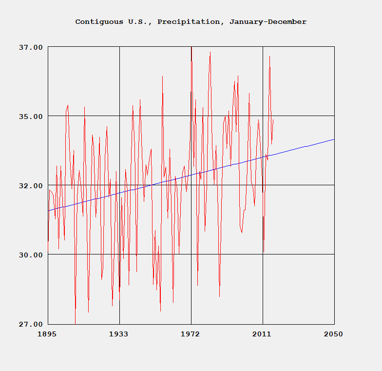
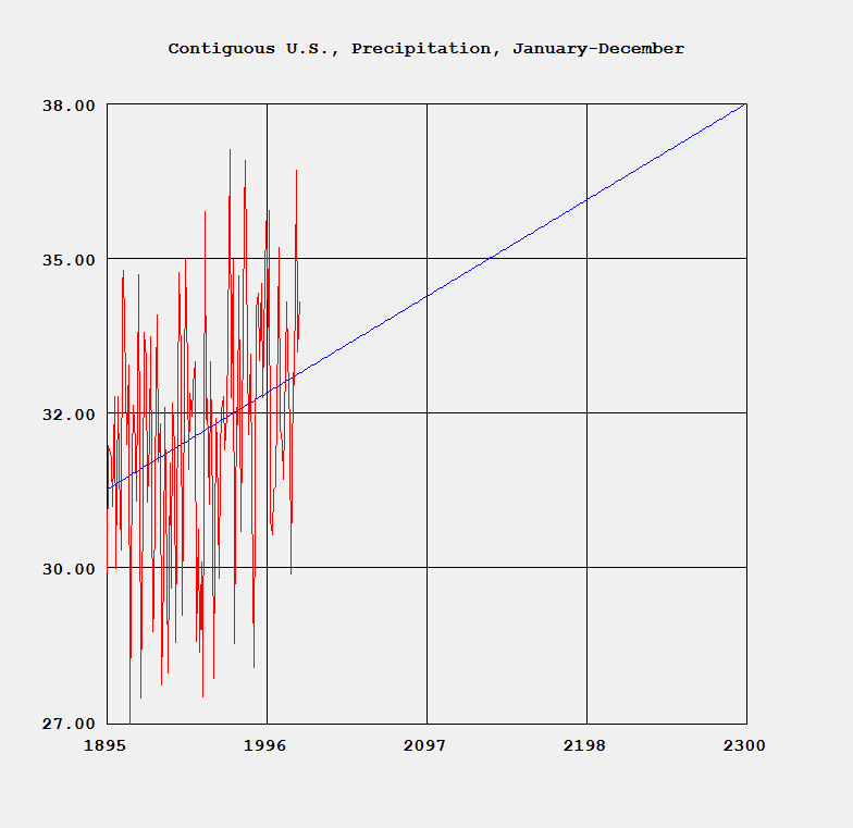
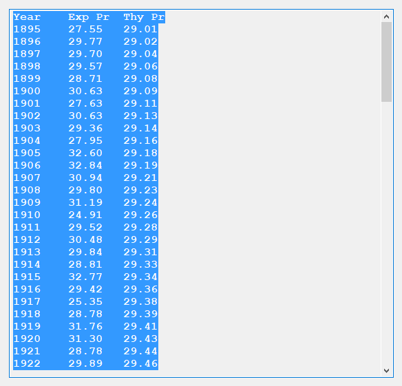
NOAA Contiguous United States of America Precipitation by James Pate Williams Jr BA, BS, MSwE, PhD
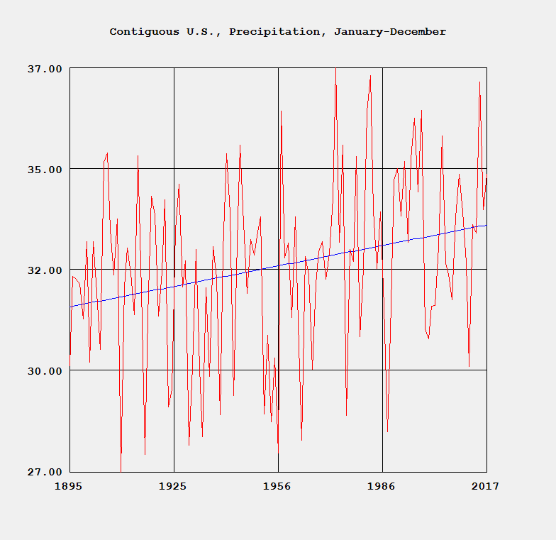
I designed and implemented a C# computer language application to model the precipitation data found on the NOAA website:
I used the latest recommended data for time period 1895 to 2017. The empirical modeling paradigm I used was simple linear regression. My model goes out to the year 2300. The key formulas used by the model are:
See the website:
https://en.wikipedia.org/wiki/Simple_linear_regression
Some plots of the contiguous U.S. precipitation are shown below. The climate is getting wetter thus some parts of the U.S.maybe more prone to floods.


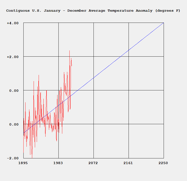
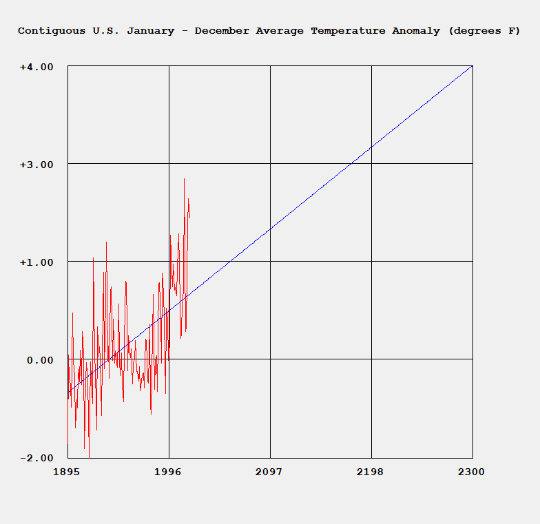
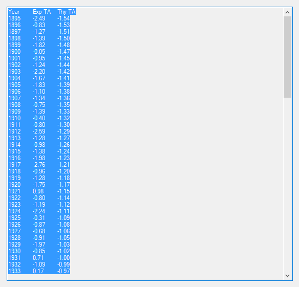
NOAA Contiguous United States of America Temperature Anomaly by James Pate Williams Jr BA, BS, MSwE, PhD
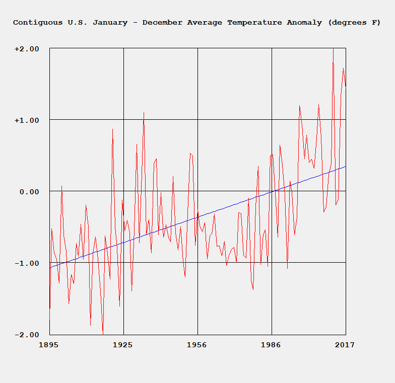
I designed and implemented a C# computer language application to model the temperature anomaly data found on the NOAA website:
I used the latest recommended data for time period 1895 to 2017. The empirical modeling paradigm I used was simple linear regression. My model goes out to the year 2300. The key formulas used by the model are:

See the website:
https://en.wikipedia.org/wiki/Simple_linear_regression
Below are some plots of the temperature anomaly.


Four Techniques for One Dimensional Riemann Definite Integration by James Pate Williams, Jr. BA, BS, MSwE, PhD
The four methods considered in this study are as follows:
- Trapezoidal Rule
- Simpson’s Rule
- Gauss-Legendre Quadrature
- Monte Carlo Method
The trapezoidal rule requires (n + 2) function evaluations, n real number increments, and six additional real number arithmetic operations. Simpson’s rule involves (n + 2) function evaluations, n real number increments, and ten additional real number arithmetic operations. Gauss-Legendre quadrature uses n function evaluations, 3 * n real number arithmetic operations, 2 * n index operations, and five additional arithmetic operations. Finally, the Monte Carlo Method requires n function evaluations, n random number generations, 2 * n + 3 additional real number arithmetic operations. The Gauss-Legendre quadrature also involves some complicated orthogonal polynomial operations to determine the abscissas and weights. Below are some results from our test C# application.


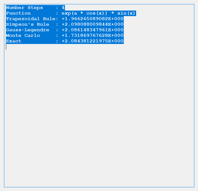
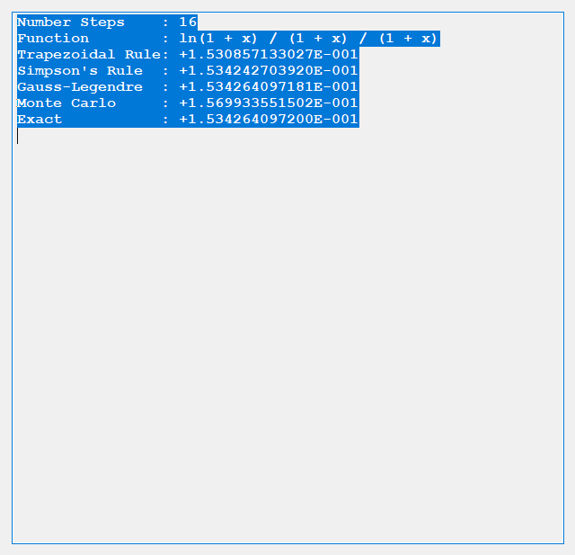

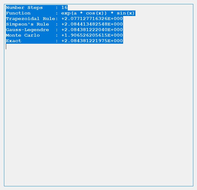

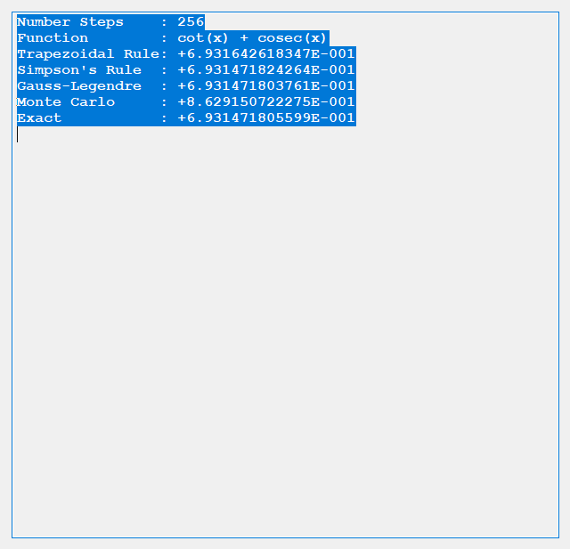

We conclude from the preceding dearth of tests that for given n the order of accuracy is generally Gauss-Legendre, Simpson’s, Trapezoidal, and finally Monte Carlo.
Calculating a Few Digits of the Transcendental Number Pi by Throwing Darts by James Pate Williams, BA, BS, MSwE, PhD
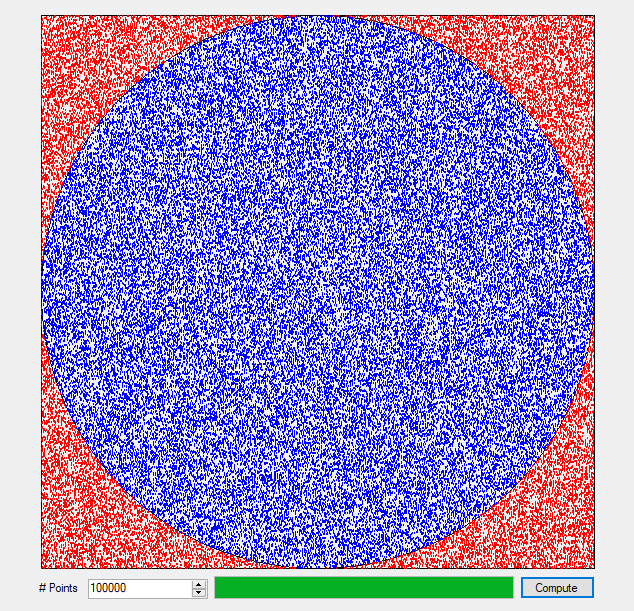
Suppose you have a unit square with a circle of unit diameter inscribed . You can compute a few digits of the transcendental number, pi, 3.1415926535897932384626433832795…, by using the algorithm described as follows. Let n be the number of darts to throw and h be the number of darts that land within the inscribed circle.
h = 0
for i = 1 to n do
Choose two random numbers x and y such that x and y are contained in the interval 0 to 1 inclusive that is x and y contained in [0, 1]
Let u = x – 1 / 2 and v = y – 1 / 2
if u * u + v * v <= 0.25 = 1 / 4 then h = h + 1
next i
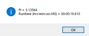
pi = 4 * h / n
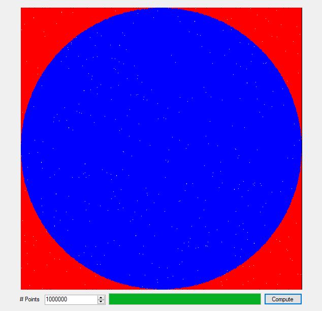
Below are the results of a C# Microsoft Visual Studio simulation project. In the first case we throw 100,000 darts and get two significant digits of pi and then we throw a 1,000,000 darts and five significant digits of pi are computed. Of course, in a previous entry by this author we can calculate hundreds or thousands of digits of pi in relatively little time: