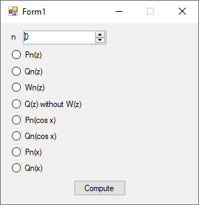
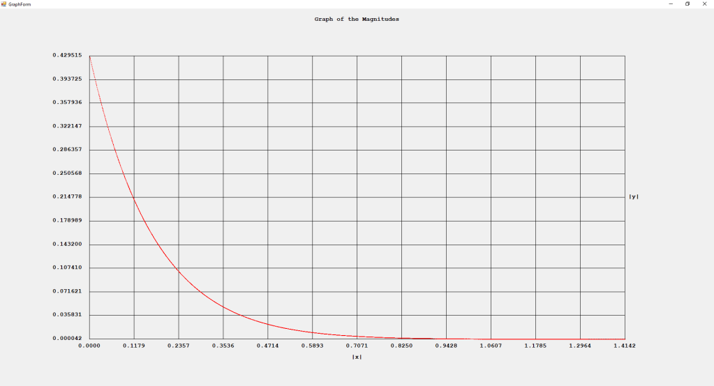
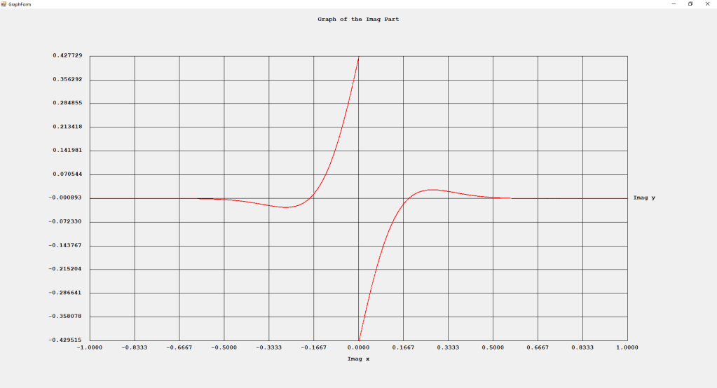
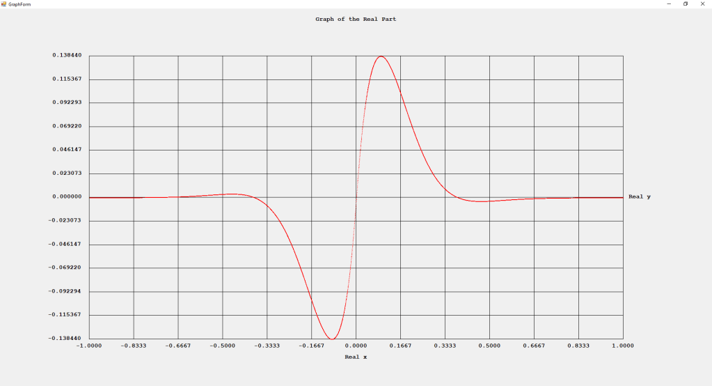
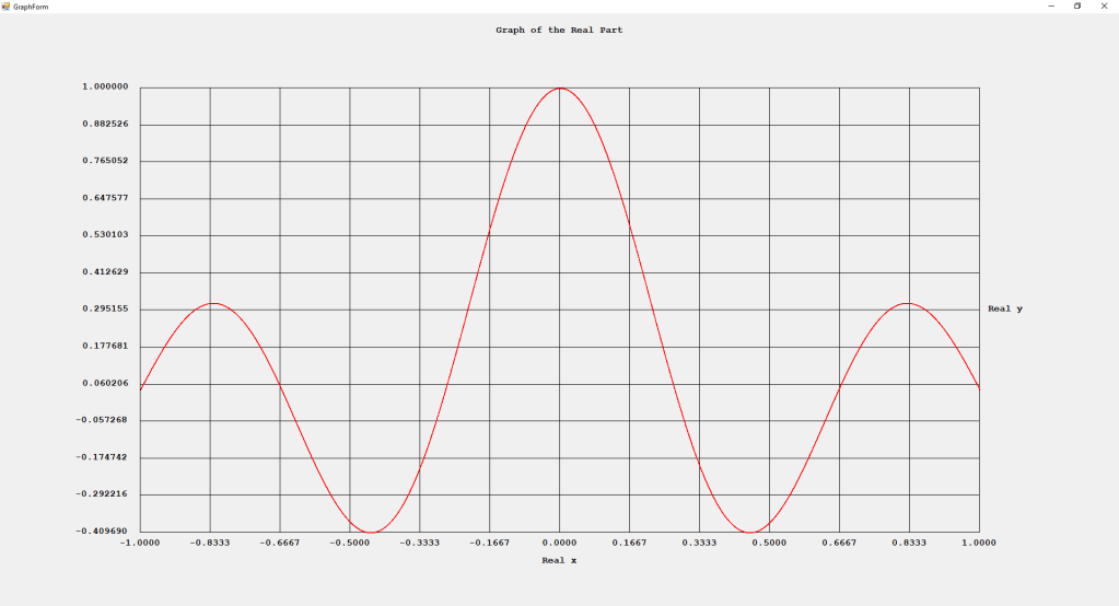
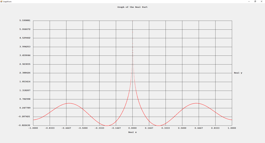
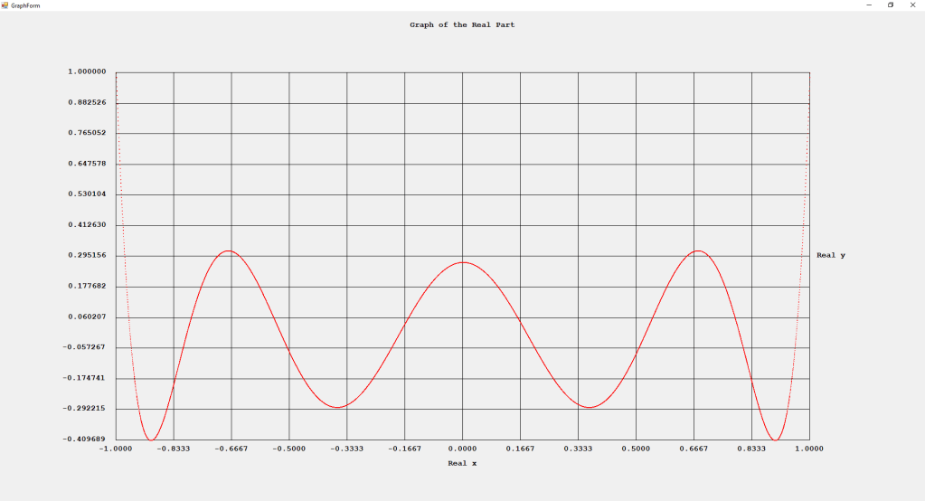
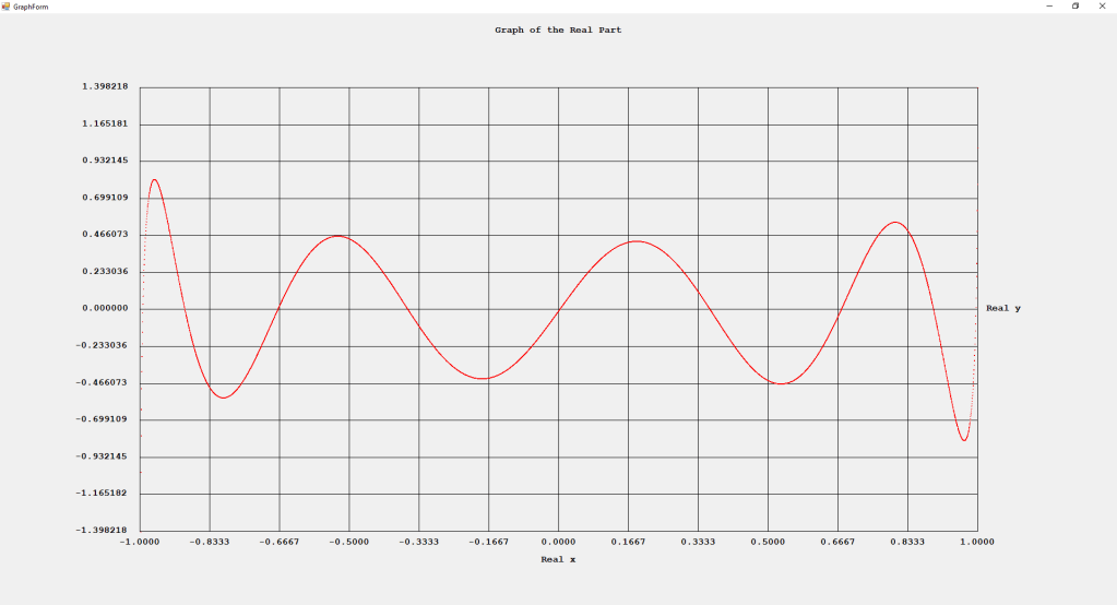
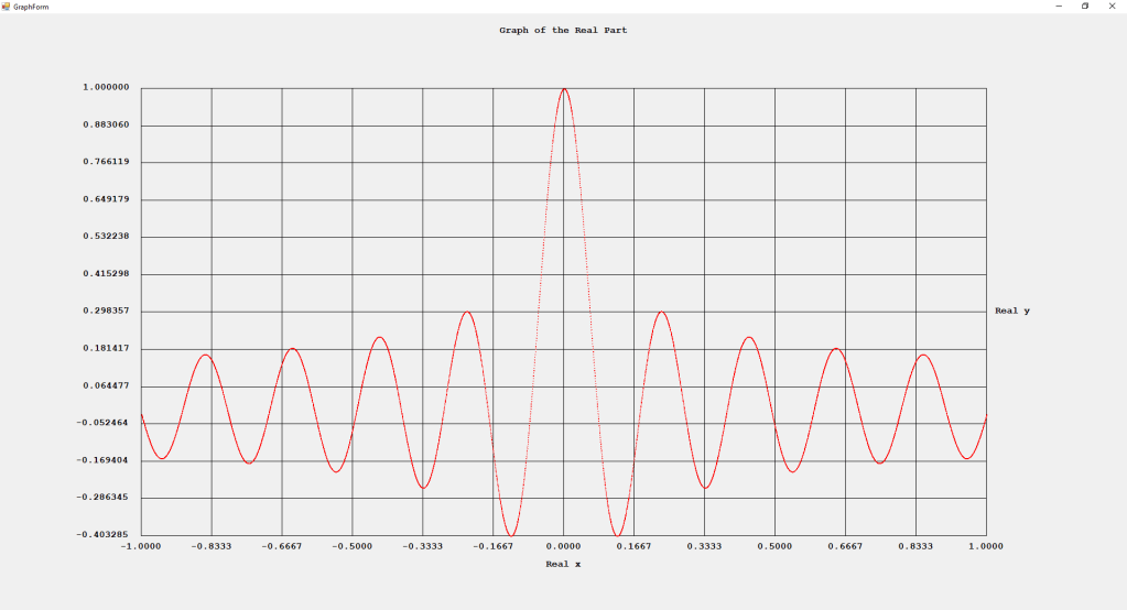
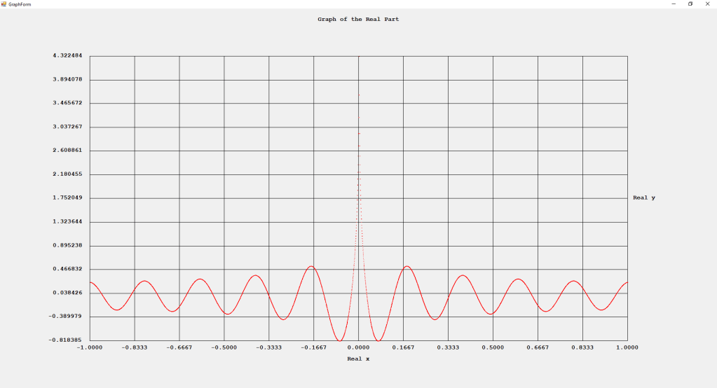
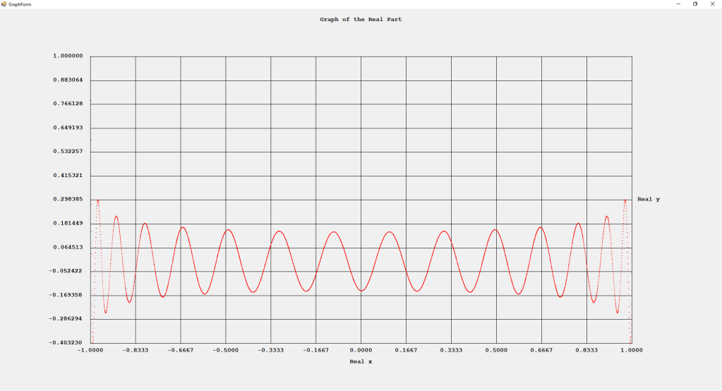
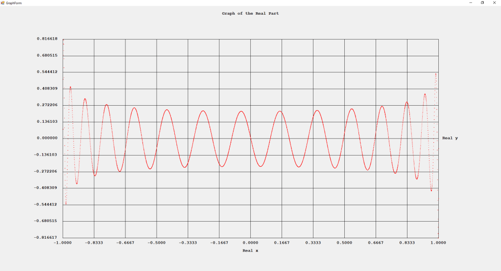
My implementations and additional graphs for the Legendre functions mentioned in the thesis cited in the preceding line and PDF. The Legendre polynomials, functions, and associated functions have many applications in quantum mechanics and other branches of applied and theoretical physics.
Legendre Functions Application
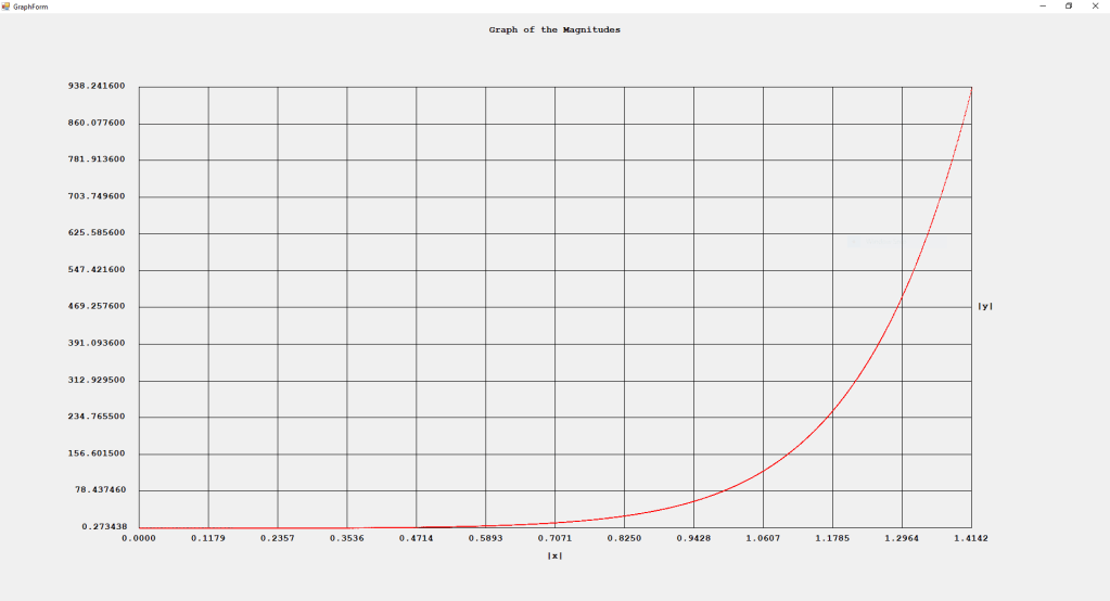
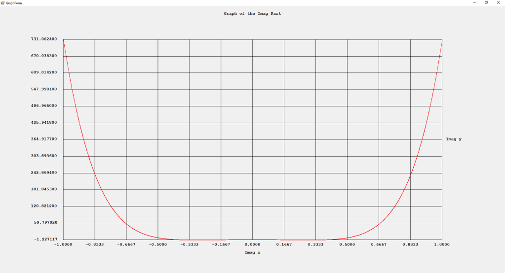
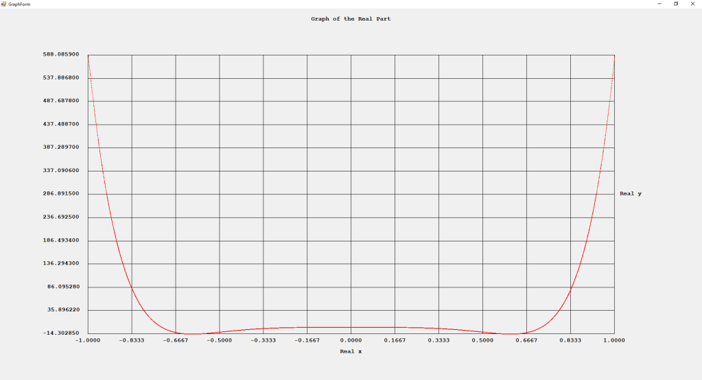
Magnitude Graph for P(z, 8)Imaginary Part for P(z, 8)Real Part for P(z, 8)Magnitudes of Q(z, 8)Imaginary Part of Q(z, 8)Real Part of Q(z, 8)Graph of P(cos x, 8) Real Valued FunctionGraph of Q(cos x, 8) Real Valued FunctionGraph of P(x, 8) Real Valued FunctionGraph of Q(x, 8) Real Valued FunctionP(cos x, 30)Q(cos x, 30)P(x, 30)Q(x, 30)
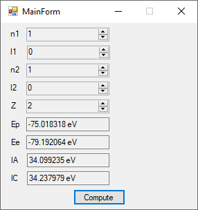
The first order perturbation calculation for the helium atom ground state is treated in detail in the textbook “Quantum Mechanics Third Edition” by Leonard I. Schiff pages 257 to 259. I offer a numerical algorithm for computing the electron-electron repulsion interaction which is analytically determined by Schiff and other scientists. Next is the graphical user interface for the application and its output.
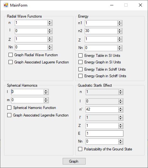
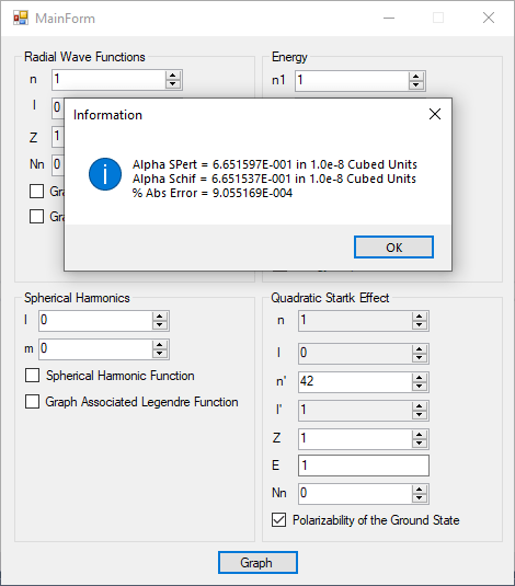
Application Graphical User Interface
The Ep text box is the ground state energy as found by a first order perturbation computation. The Ee text box is the experimental ground state energy. The IA text box is the analytic electron-electron repulsion interaction determined by Schiff and other quantum mechanics researchers. The IC text box is my numerical contribution. All the energies are in electron volts.
The application source code are the next items in this blog.
In my current return to my youthful dual interests in quantum chemistry and quantum mechanics that occupied much of my time in the 1960s, 1970s and 1980s, I am now using my knowledge of experimental numerical analysis. My interest in computer science and numerical analysis began in the summer of 1976 while I was a chemistry student at my local college namely LaGrange College in LaGrange, Georgia. As a child and teenager I was very interested in several disciplines of physics: classical mechanics, quantum mechanics, and the theories of special and general relativity. Later I added to my knowledge toolkit some tidbits of statistical mechanics and statistical thermodynamics.
This blog entry will explore the wonderful world of the hydrogenic atom which used to known by the moniker, hydrogen-like atom. The most well known isotope of hydrogen has one electron and one proton and its atomic number is 1 and it is sometimes denoted by the letter and numeral Z = 1. Of course, there are multiple other isotopes of hydrogen including deuterium (one proton and one neutron) and tritium (one proton and two neutrons). Hydrogen is the only atom whose wave functions both non-relativistic (see Erwin Schrödinger) and relativistic (view Paul Adrian Maurice Dirac) have analytic close formed solutions. Hydrogen is the most abundant chemical element on Earth and in the universe. The stars initially use a hydrogen plasma as a nuclear fuel to create more massive atomic ions and release massive amounts of nuclear fusion energy.
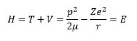
Way back in the 1920s Erwin Schrödinger decided to apply his work in wave hydrology to the newly found branch of physics known as quantum theory and quantum mechanics. From his work the branch of quantum mechanics known as wave quantum mechanics evolved. This branch was as important as another competing theory of quantum mechanics known as matrix quantum mechanics that was being concurrently developed by Werner Heisenberg. The key process in the derivation of a Schrödinger equation for any time independent scenario is to apply the first quantization rules to a valid classical Hamiltonian. The classical Hamiltonian is the total energy of a system and is the sum of the kinetic energy and the potential energy. The classical Hamiltonian for the hydrogen-like atom is shown in equation (1).
Equation (1), Many Sources
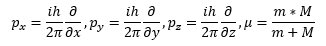
The first quantization rule is to apply the conversion from a classical momentum vector to a momentum quantum mechanical operator using the equation (2).
Equation (2), Several Sources
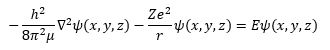
The lower case m is the mass of the electron and the upper case M is the mass of the atomic nucleus which is the Z times the proton mass plus the number of neutrons times the neutron mass. The Greek letter mu is the reduced mass of the hydrogen-like system. The italic i is the imaginary unit that is the square root of the number -1. The transcendental number pi is represented by the Greek letter pi and has the truncated real number value of 3.1415926535897932384626433832795. Schrödinger plugged Equation (2) into Equation (1) and found a three-dimensional Cartesian coordinate second order partial differential equation (3) that used the operator discovered by the mathematician Laplace.
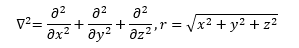
Equation (3), Merzbacher, Messiah, Schiff Et. Al.Equation (4), Several Sources
In equation (4) the first partial differential operator is the Laplace operator which is the vector inner product of the three-dimensional Cartesian gradient operator from vector analysis. The scalar r in equation (4) is the Euclidean distance from the electron to the nucleus. The Greek letter psi (“pitchfork”) in equation (3) is the illustrious and elusive wave function.
The first thing that struck Schrödinger was that the equation (3) that he derived by much thought was unfortunately not a separable partial differential equation in three-dimensional Cartesian coordinates, however, he next applied a coordinate coordinate transformation from three-dimensional Cartesian coordinates to three dimensional spherical polar equations specified by the equations in the following PDF with some derivations.
The wave function for the hydrogen-like atom is dependent on the associated Laguerre polynomials and the spherical harmonics that dependent upon the associated Legendre functions.
using System;

namespace SteadyStateTempCylinder
{
    public class PotPoint : IComparable
    {
        private double x, y, u;

        public double X
        {
            get
            {
                return x;
            }
            set
            {
                x = value;
            }
        }

        public double Y
        {
            get
            {
                return y;
            }
            set
            {
                y = value;
            }
        }

        public double U
        {
            get
            {
                return u;
            }
            set
            {
                u = value;
            }
        }

        public PotPoint(double x, double y, double u)
        {
            this.x = x;
            this.y = y;
            this.u = u;
        }

        public int CompareTo(object obj)
        {
            if (obj == null)
                return 1;

            PotPoint pp = (PotPoint)obj;

            if (u > pp.u)
                return 1;
            else if (u == pp.u)
                return 0;
            else
                return -1;
        }
    }
}
The description of this alphabetic letter game is very facile. Given a word make as many other words as possible using the letters of the given initial word. But first before we enumerate the game solution, we need to refresh the reader’s memory of some elementary mathematics.
The binary number system also known as the base 2 number system is used by computers to perform arithmetic. The digits in the binary number system are 0 and 1. The numbers 0 to 15 in binary using only four binary digits are where ^ is the exponentiation operator (raising a number to a power) are:
0	0000
1	0001	2 ^ 0 = 1
2	0010	2 ^ 1 = 2
3	0011	2 ^ 1 + 2 ^ 0 = 2 + 1 = 3
4	0100	2 ^ 2 = 4
5	0101	2 ^ 2 + 2 ^ 0 = 4 + 1 = 5
6	0110	2 ^ 2 + 2 ^ 1 = 4 + 2 = 6
7	0111	2 ^ 2 + 2 ^ 1 + 2 ^ 0 = 4 + 2 + 1 = 7
8	1000	2 ^ 3 = 8
9	1001	2 ^ 3 + 2 ^ 0 = 8 + 1 = 9
10	1010	2 ^ 3 + 2 ^ 1 = 8 + 2 = 10
11	1011	2 ^ 3 + 2 ^ 1 + 2 ^ 0 = 8 + 2 + 1 = 11
12	1100	2 ^ 3 + 2 ^ 2 = 8 + 4 = 12
13	1101	2 ^ 3 + 2 ^ 2 + 2 ^ 0 = 8 + 4 + 1 = 13
14	1110	2 ^ 3 + 2 ^ 2 + 2 ^ 1 = 8 + 4 + 2 = 14
15	1111	2 ^ 3 + 2 ^ 2 + 2 ^ 1 + 2 ^ 0 = 8 + 4 + 2 + 1 = 15

An algorithm to convert a base 10 (decimal) number to base 2 (binary) number is given below:
Input n a base 10 number
Output b[0], b[1], b[2], … a finite binary string representing the decimal number

Integer i = 0

Do
Integer nmod2 = n mod 2
Integer ndiv2 = n / 2

b[i] = nmod2 + ‘0’
i = i + 1

n = ndiv2

While n > 0

The b[i] will be in reverse order. For example, convert 12 from decimal to using four binary digits:
12 mod 2 = 0
12 div 2 = 6

b[0] = ‘0’

i = 1

n = 6

6 mod 2 = 0
6 div 2 = 3

b[1] = ‘0’

i = 2

n = 3

3 mod 2 = 1
3 div 2 = 1

i = 3

b[2] = ‘1’

n = 1

1 mod 2 = 1
1 div 2 = 0

b[3] = ‘1’

n = 0

So, the reversed binary string of digits is “0011”. And after reversing the string we have 12 is represented by the binary digits “1100”.

Next, we need to define a power set and its binary representation. The index power set of 4 objects which has 2 ^ 4 = 16 entries is specified in the following table:
0	0000
1	0001
2	0010
3	0011
4	0100
5	0101
6	0110
7	0111
8	1000
9	1001
10	1010
11	1011
12	1100
13	1101
14	1110
15	1111
A permutation of the set of three indices is given by the following list:
012, 021, 102, 120, 201, 210

A permutation of n objects is a list of n! = n * (n – 1) * … * 2 * 1. A permutation of 4 objects has a list of 24 – 4-digit indices list since 4! = 4 * 3 * 2 * 1 = 24 has the table:
0123, 0132, 0213, 0231, 0312, 0321,
1023, 1032, 1203, 1230, 1320, 1302,
2013, 2031, 2103, 2130, 2301, 2310,
3012, 3021, 3102, 3120, 3201, 3210

Suppose our word is “lost” then we first find the power set:

1	0001	t
2	0010	s
3	0011	st	ts
4	0100	o
5	0101	ot	to
6	0110	os	so
7	0111	ost	ots	sot	sto	tos	tso
8	1000	l
9	1001	lt	tl
10	1010	ls	sl
11	1011	lst	lts	slt	stl	tsl	tls
12	1100	lo	ol
13	1101	lot	lto	olt	otl	tlo	tol
14	1110	los	lso	slo	sol	osl	ols
15	1111	lost	lots	slot	etc.

Using a dictionary of 152,512 English words my program finds 16 hits for the letters of “lost”:

Dictionary Length: 152512

Word: lost

  0     l
  1     lo
  2     lost
  3     lot
  4     lots
  5     ls
  6     o
  7     s
  8     slot
  9     so
 10     sol
 11     sot
 12     st
 13     t
 14     to
 15     ts

Total letters and/or words 16

Next, we use “tear” as our word:

Dictionary Length: 152512

Word: tear

  0     a
  1     are
  2     art
  3     at
  4     ate
  5     e
  6     ea
  7     ear
  8     eat
  9     era
 10     et
 11     eta
 12     r
 13     rat
 14     rate
 15     re
 16     rt
 17     rte
 18     t
 19     tar
 20     tare
 21     tea
 22     tear
 23     tr

Total letters and/or words 24

Finally, we use the word “company”:

Dictionary Length: 152512

Word: company

  0     a
  1     ac
  2     am
  3     amp
  4     an
  5     any
  6     c
  7     ca
  8     cam
  9     camp
 10     campy
 11     can
 12     canopy
 13     cap
 14     capo
 15     capon
 16     cay
 17     cm
 18     co
 19     com
 20     coma
 21     comp
 22     company
 23     con
 24     cony
 25     cop
 26     copay
 27     copy
 28     coy
 29     cyan
 30     m
 31     ma
 32     mac
 33     man
 34     many
 35     map
 36     may
 37     mayo
 38     mo
 39     moan
 40     mop
 41     mp
 42     my
 43     myna
 44     n
 45     nap
 46     nay
 47     nm
 48     no
 49     o
 50     om
 51     on
 52     op
 53     p
 54     pa
 55     pan
 56     pay
 57     pm
 58     pony
 59     y
 60     ya
 61     yam
 62     yap
 63     yo
 64     yon

Total letters and/or words 65

The C++ program's source code is given below:

// WordToWords.cpp : This file contains the 'main' function. Program execution begins and ends there.
//

#include "pch.h"
#include <algorithm>
#include <fstream>
#include <iomanip>
#include <iostream>
#include <string>
#include <vector>

using namespace std;

vector<string> dictWords;

bool ReadDictionaryFile()
{
    fstream newfile;

    newfile.open("C:\\Users\\james\\source\\repos\\WordToWords\\Dictionary.txt", ios::in);

    if (newfile.is_open()) {
        int index = 0, length = 128;
        char cstr[128];

        while (newfile.getline(cstr, length)) {
            string str;

            str.clear();

            for (int i = 0; i < (int)strlen(cstr); i++)
                str.push_back(cstr[i]);

            dictWords.push_back(str);
        }

        newfile.close();

        sort(dictWords.begin(), dictWords.end());
        return true;
    }

    else
        return false;
}

string ConvertBase2(char cstr[], int n, int len)
{
    int count = 0;
    string str, rev;

    do
    {
        int nMod2 = n % 2;
        int nDiv2 = n / 2;

        str.push_back(nMod2 + '0');
        n = nDiv2;
    } while (n > 0);

    n = str.size();

    for (int i = n; i < len; i++)
        str.push_back('0');

    n = str.size();

    for (int i = n - 1; i >= 0; i--)
        if (str[i] == '1')
            rev.push_back(cstr[i]);

    return rev;
}

vector<string> PowerSet(char cstr[], int len)
{
    vector<int> index;
    vector<string> match;

    for (long ps = 0; ps <= pow(2, len); ps++)
    {
        string str = ConvertBase2(cstr, ps, len);
        int psf = 1;

        for (int i = 2; i <= len; i++)
            psf *= i;

        for (int i = 0; i < psf; i++)
        {
            if (binary_search(dictWords.begin(), dictWords.end(), str))
            {
                if (!binary_search(match.begin(), match.end(), str))
                {
                    match.push_back(str);
                    sort(match.begin(), match.end());
                }
            }

            next_permutation(str.begin(), str.end());
        }

        sort(match.begin(), match.end());
    }

    return match;
}

int main()
{
    bool done = false;
    char cstr[128];
    int len;
    string str;
    vector<int> index;
    vector<string> match;

    if (!ReadDictionaryFile())
        return -1;

    cout << "Dictionary Length: " << dictWords.size() << endl << endl;

    cout << "Word: ";
    cin >> cstr;
    cout << endl;

    len = strlen(cstr);

    if (len != 0)
    {
        vector<string> match = PowerSet(cstr, len);

        for (int i = 0; i < match.size(); i++)
        {
            cout << setprecision(3) << setw(3) << i << "\t";
            cout << match[i] << endl;
        }

        cout << endl;
        cout << "Total letters and/or words " << match.size() << endl;
        cout << endl;
    }
}