My whole legal name is James Pate Williams, Jr. I was born in LaGrange, Georgia approximately 70 years ago. I barely graduated from LaGrange High School with low marks in June 1971. Later in June 1979, I graduated from LaGrange College with a Bachelor of Arts in Chemistry with a little over a 3 out 4 Grade Point Average (GPA). In the Spring Quarter of 1978, I taught myself how to program a Texas Instruments desktop programmable calculator and in the Summer Quarter of 1978 I taught myself Dayton BASIC (Beginner's All-purpose Symbolic Instruction Code) on LaGrange College's Data General Eclipse minicomputer. I took courses in BASIC in the Fall Quarter of 1978 and FORTRAN IV (Formula Translator IV) in the Winter Quarter of 1979. Professor Kenneth Cooper, a genius poly-scientist taught me a course in the Intel 8085 microprocessor architecture and assembly and machine language. We would hand assemble our programs and insert the resulting machine code into our crude wooden box computer which was designed and built by Professor Cooper. From 1990 to 1994 I earned a Bachelor of Science in Computer Science from LaGrange College. I had a 4 out of 4 GPA in the period 1990 to 1994. I took courses in C, COBOL, and Pascal during my BS work. After graduating from LaGrange College a second time in May 1994, I taught myself C++. In December 1995, I started using the Internet and taught myself client-server programming. I created a website in 1997 which had C and C# implementations of algorithms from the "Handbook of Applied Cryptography" by Alfred J. Menezes, et. al., and some other cryptography and number theory textbooks and treatises.
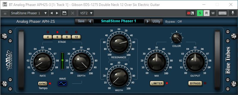
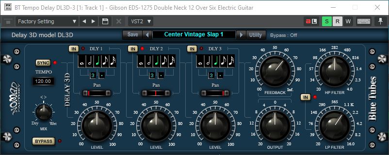
Gibson EDS-1275 Double Neck Twelve String Over Six String Guitar May 2009 Post Production March 2022
Gibson EDS-1275 Double Neck Twelve String Over Six String Guitar May 2009 Post Production March 2022First Effect for First Video of this Blog EntrySecond Effect for First Video of this Blog EntryThird Effect for First Video of this Blog EntryFourth Effect for First Video of this Blog EntryFifth Effect for First Video of this Blog EntryEffects Used in the Second Video
Windows ’95 MIDI Sequencer Translated from Java in About 2005
An Early Attempt at Creating Computer Generated Music in May 1988 Using My Brand New Commodore Amiga 2000 and Microsoft’s Amiga Basic The Amiga’s Display Uses Colors but my 2015 Recreation Is in Black and White (Monochrome)