Category: Elementary Physics
Partial Solution to a Neat Problem from an Online Textbook
Some Helium Coulomb Integrals over Six Dimensions by James Pate Williams, Jr. Source Code in C++ Development over December 15 – 16, 2023
Revised Translated Source Code from May 15, 2015, by James Pate Williams, Jr.
New and Corrected Ground State Energy Numerical Computation for the Helium Like Atom (Atomic Number 2) by James Pate Williams, Jr.
A New Calculus of Variations Solution of the Schrödinger Equation for the Lithium Like Atom’s Ground State Energy
This computation took a lot longer time to reach a much better solution than my previously published result.
Guitar String and Piano Key Frequencies by James Pate Williams, Jr.
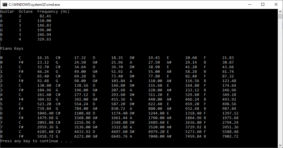
// FrequencyKey.cpp : Defines the entry point for the console application.
// James Pate Willims, Jr. (c) All Applicable Rights Reserved

#include "stdafx.h"
#include <math.h>
#include <iomanip>
#include <iostream>
#include <string>
#include <vector>
using namespace std;

vector<string> pnote;
double a = pow(2.0, 1.0 / 12.0);
double f0 = 440.0, gStrF[6];
double e2, a2, d3, g3, b3, e4;
double pfreq[9 * 12];
int offset = 0;

double fn(int n)
{
	return f0 * pow(a, n);
}

void printFrequency(char note, int octave, double frequency)
{
	cout << note << "\t" << octave << "\t";
	cout << setw(6) << fixed << setprecision(2);
	cout << frequency << endl;
}

int main()
{
	for (int octave = 0; octave <= 8; octave++)
	{
		pnote.push_back("C");
		pnote.push_back("C#");
		pnote.push_back("D");
		pnote.push_back("D#");
		pnote.push_back("E");
		pnote.push_back("F");
		pnote.push_back("F#");
		pnote.push_back("G");
		pnote.push_back("G#");
		pnote.push_back("A");
		pnote.push_back("A#");
		pnote.push_back("B");
	}

	pfreq[0] = 16.35;
	pfreq[1] = 17.32;
	pfreq[2] = 18.35;
	pfreq[3] = 19.45;
	pfreq[4] = 20.6;
	pfreq[5] = 21.83;
	pfreq[6] = 23.12;
	pfreq[7] = 24.5;
	pfreq[8] = 25.96;
	pfreq[9] = 27.5;
	pfreq[10] = 29.14;
	pfreq[11] = 30.87;

	for (int octave = 1; octave <= 8; octave++)
	{
		for (int i = 0; i < 12; i++)
		{
			pfreq[octave * 12 + i] = 2.0 * pfreq[(octave - 1) * 12 + i];
		}
	}

	gStrF[0] = e2 = fn(offset - 29);
	gStrF[1] = a2 = fn(offset - 24);
	gStrF[2] = d3 = fn(offset - 19);
	gStrF[3] = g3 = fn(offset - 14);
	gStrF[4] = b3 = fn(offset - 10);
	gStrF[5] = e4 = fn(offset - 5);

	cout << "Guitar\tOctave\tFrequency (Hz)" << endl;

	printFrequency('E', 2, e2);
	printFrequency('A', 2, a2);
	printFrequency('D', 3, d3);
	printFrequency('G', 3, g3);
	printFrequency('B', 3, b3);
	printFrequency('E', 4, e4);

	cout << endl;
	cout << "Piano Keys" << endl << endl;

	for (int octave = 0; octave <= 8; octave++)
	{
		for (int i = 0; i < 2; i++)
		{
			cout << octave << '\t';

			for (int j = 0; j < 6; j++)
			{
				{
					cout << pnote[(12 * octave + 6 * i + j) % 12] << '\t';
					cout << pfreq[(12 * octave + 6 * i + j)] << '\t';
				}
			}

			cout << endl;
		}
	}

	return 0;
}
Two of Kepler’s Three Laws of Planetary Motion by James Pate Williams, Jr.
Derivation of de Broglie’s Wave-Particle Duality Principle of Quantum Mechanics and Macroscopic Exercise by James Pate Williams, Jr.
Estimated Babe Ruth 1921 Homerun Parameters by James Pate Williams, Jr.
“Babe Ruth is generally considered the owner of the record for the longest home run in MLB history with a 575-foot bomb launched at Navin Field in Detroit in 1921.” – https://www.msn.com/en-us/sports/mlb/what-is-the-longest-home-run-in-mlb-history/ar-AA1dGwlZ
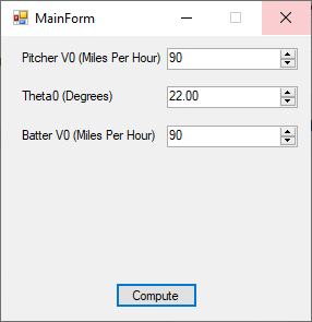
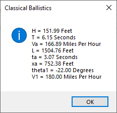
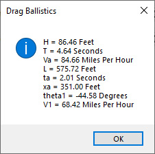
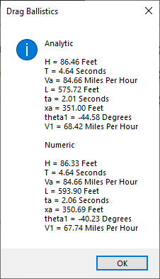
As you can see, I estimated the pitch velocity at 90 miles per hour and Babe Ruth’s (Sultan of Swing) at 90 miles per hour also. My analytic calculations yield a range of the baseball’s trajectory as about 576 feet.
