Category: Complex Functions
Blog Entry © Tuesday, October 29, 2024, by James Pate Williams, Jr. Second Order Quantum Mechanical Perturbation Calculation Part I
Blog Entry © Monday, October 14, 2024, Real Eigenvalues and Eigenvectors of a 4 x 4 Tridiagonal Matrix and Solutions of a 4 x 4 System Using the Same Tridiagonal Matrix by James Pate Williams, Jr.
Two methods of solving linear systems of equations are explored in this blog. The methods are the Gauss-Seidel method and the Jacobi iteration.
Blog Entry © Tuesday, October 8, 2024, by James Pate Williams, Jr.
Blog Entry (c) Wednesday, October 2, 2024, by James Pate Williams, Jr. First Order Coupled Ordinary Differential Equations
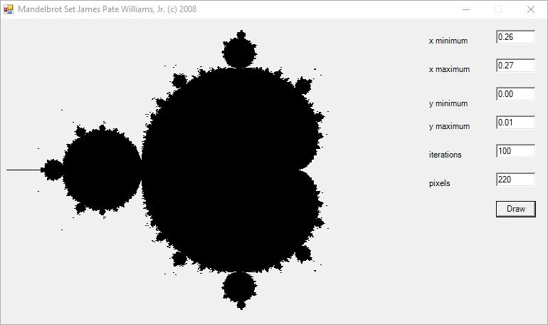
Blog Entry (c) Saturday, September 14, 2024, The Mandelbrot Set by James Pate Williams, Jr. A Simple Fractal Self-Similar Curve
Blog Entry (c) Tuesday, July 23, 2024, by James Pate Williams, Jr. Mueller’s Method for Finding the Complex and/or Real Roots of a Complex and/or Real Polynomial
I originally implemented this algorithm in FORTRAN IV in the Summer Quarter of 1982 at the Georgia Institute of Technology. I was taking a course named “Scientific Computing I” taught by Professor Gunter Meyer. I made a B in the class. Later in 2015 I re-implemented the recipe in C# using Visual Studio 2008 Professional. VS 2015 did not have support for complex numbers nor large integers. In December of 2015 I upgraded to Visual Studio 2015 Professional which has support for big integers and complex numbers. I used Visual Studio 2019 Community version for this project. Root below should be function.
Degree (0 to quit) = 2
coefficient[2].real = 1
coefficient[2].imag = 0
coefficient[1].real = 1
coefficient[1].imag = 0
coefficient[0].real = 1
coefficient[0].imag = 0

zero[0].real = -5.0000000000e-01        zero[0].imag =  8.6602540378e-01
zero[1].real = -5.0000000000e-01        zero[1].imag = -8.6602540378e-01

root[0].real =  0.0000000000e+00        root[0].imag = -2.2204460493e-16
root[1].real =  3.3306690739e-16        root[1].imag = -7.7715611724e-16

Degree (0 to quit) = 3
coefficient[3].real = 1
coefficient[3].imag = 0
coefficient[2].real = 0
coefficient[2].imag = 0
coefficient[1].real = -18.1
coefficient[1].imag = 0
coefficient[0].real = -34.8
coefficient[0].imag = 0

zero[0].real = -2.5026325486e+00        zero[0].imag = -8.3036679880e-01
zero[1].real = -2.5026325486e+00        zero[1].imag =  8.3036679880e-01
zero[2].real =  5.0052650973e+00        zero[2].imag =  2.7417672687e-15

root[0].real =  0.0000000000e+00        root[0].imag =  1.7763568394e-15
root[1].real =  3.5527136788e-14        root[1].imag = -1.7763568394e-14
root[2].real =  2.8421709430e-14        root[2].imag =  1.5643985575e-13

Degree (0 to quit) = 5
coefficient[5].real = 1
coefficient[5].imag = 0
coefficient[4].real = 2
coefficient[4].imag = 0
coefficient[3].real = 3
coefficient[3].imag = 0
coefficient[2].real = 4
coefficient[2].imag = 0
coefficient[1].real = 5
coefficient[1].imag = 0
coefficient[0].real = 6
coefficient[0].imag = 0

zero[0].real = -8.0578646939e-01        zero[0].imag =  1.2229047134e+00
zero[1].real = -8.0578646939e-01        zero[1].imag = -1.2229047134e+00
zero[2].real =  5.5168546346e-01        zero[2].imag =  1.2533488603e+00
zero[3].real =  5.5168546346e-01        zero[3].imag = -1.2533488603e+00
zero[4].real = -1.4917979881e+00        zero[4].imag =  1.8329656063e-15

root[0].real =  8.8817841970e-16        root[0].imag =  4.4408920985e-16
root[1].real = -2.6645352591e-15        root[1].imag = -4.4408920985e-16
root[2].real =  8.8817841970e-16        root[2].imag =  1.7763568394e-15
root[3].real =  3.4638958368e-14        root[3].imag = -1.4210854715e-14
root[4].real =  8.8817841970e-16        root[4].imag =  2.0710031449e-14
Blog Entry Friday, June 14, 2024 (c) James Pate Williams, Jr.
For the last week or so I have been working my way through Chapter 3 The Solution of Nonlinear Equations found in the textbook “Numerical Analysis: An Algorithmic Approach” by S. D. Conte and Carl de Boor. I also used some C source code from “A Numerical Library in C for Scientists and Engineers” by H. T. Lau, PhD. I implemented twenty examples and exercises from the previously mentioned chapter.
Complex Number Calculator © March 25-26 by James Pate Williams, Jr.
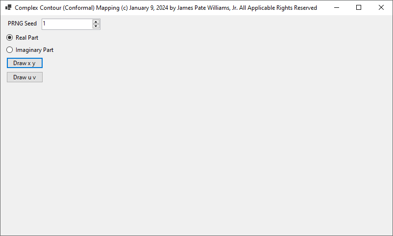
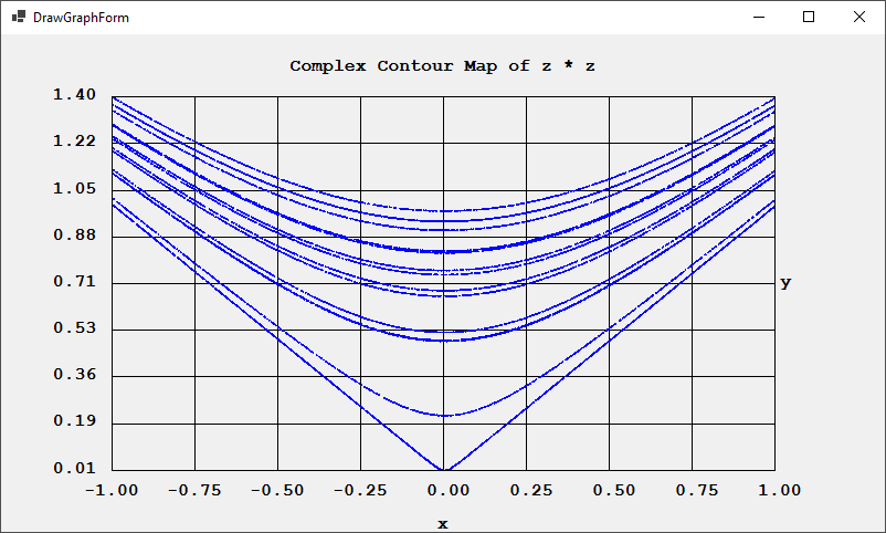
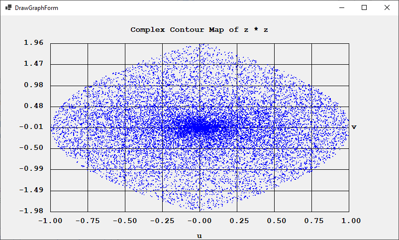
Complex Contour (Conformal) Mapping by James Pate Williams, Jr. on January 9, 2024