Category: Elementary Physics
Blog Entry, Thursday, March 20, 2025, Another Helium Variational Calculation by James Pate Williams, Jr.
Blog Entry, Tuesday, March 18, 2025, Problems from the Textbook: Mathematical Methods in the Physical Sciences Second Edition © 1983 by Mary L. Boas, Solutions Provided by James Pate Williams, Jr.
Blog Entry, Monday, March 10, 2025, Problems from the Textbook: Mathematical Methods in the Physical Sciences Second Edition © 1983 by Mary L. Boas, Solutions Provided by James Pate Williams, Jr.
Ground State Energies of the Hydrogen Molecule and Hydrogen Molecular Ion by James Pate Williams, Jr., BA, BS, Master of Software Engineering, PhD Computer Scienc
Solution of the Fermi-Thomas Potential Energy Equation for Zero Temperature and without Exchange by James Pate Williams, Jr.
Exercises from Elementary Statistical Physics by C. Kittel by James Pate Williams, Jr.
More Results from the 1953 Metropolis Among Others Technical Report © Tuesday, February 25, 2025, by James Pate Williams, Jr.
Reproduction and Extension of Metropolis Among Others Results in Their 1953 Technical Report (c) February 22, 2025, by James Pate Williams, Jr.
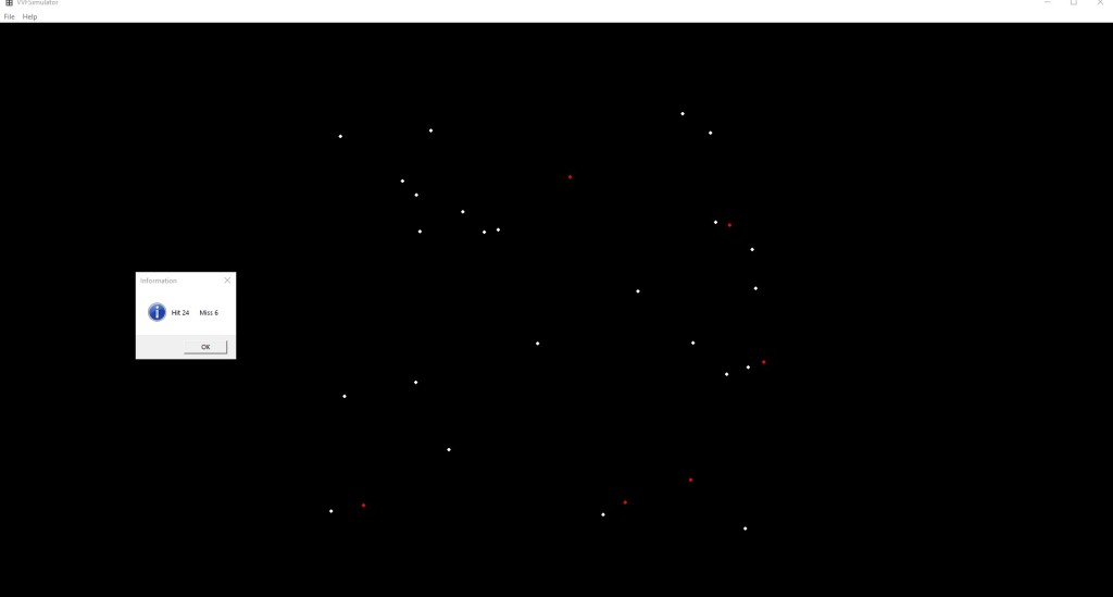
Blog Entry © Saturday, January 18, 2025, by James Pate Williams, Jr. Preliminary Virtual Vision Field (VVF) Diagnostic Optometry Test Simulator
I was administered a VVF Test on Wednesday, January 15, at Dr. Brent Brown and Associates Inc office in LaGrange, Georgia. The test consists of using a headset that has an orange circle in the center of the display. The examinee has a trigger device to click each time a white flash occurs. I decided to write a C/C++ Win32 application to simulate the VVF Test. The following two pictures are from a simulated test of one minute in duration. The white flashes are separated by 1000 millisecond (1 second) and their durations are also 1000 milliseconds (1 second).
Positions of the Hits
1 (571, 842)
2 (587, 196)
3 (594, 644)
4 (694, 273)
5 (717, 620)
6 (718, 297)
7 (724, 360)
8 (743, 186)
9 (774, 736)
10 (798, 326)
11 (835, 361)
12 (859, 357)
13 (927, 553)
14 (1040, 848)
15 (1100, 463)
16 (1177, 157)
17 (1195, 552)
18 (1225, 190)
19 (1234, 344)
20 (1253, 606)
21 (1285, 872)
22 (1290, 594)
23 (1297, 391)
24 (1303, 458)
Positions of the Misses
1 (627, 832)
2 (983, 266)
3 (1078, 827)
4 (1191, 788)
5 (1258, 349)
6 (1317, 585)
