Some modern physical models of our universe require more than Einstein’s four dimensions: three spatial dimensions and one time dimension. Why do people worry about introducing more dimensions into our understanding of chemistry and physics? When Erwin Schrödinger introduced his famous quantum mechanical two-body solution of the time independent hydrogen-like atom wave equation he went four dimensions to three spatial dimensions. Later, Wolfgang Pauli espoused his famous Pauli Exclusion Principle that simply stated no two electrons (fermions) in an atomic orbital can have the same quantum spin number. Atoms live in a four-dimensional quantum number space augmented by three spatial dimensions and one time dimension.
Category: Quantum Mechanics and Quantum Chemistry
Revised Translated Source Code from May 15, 2015, by James Pate Williams, Jr.
A New Calculus of Variations Solution of the Schrödinger Equation for the Lithium Like Atom’s Ground State Energy
This computation took a lot longer time to reach a much better solution than my previously published result.
A Calculus of Variations Solution to the Quantum Mechanical Schrödinger Wave Equation for the Lithium Like Atom (Atomic Number Z = 3) by James Pate Williams, Jr.
Derivation of de Broglie’s Wave-Particle Duality Principle of Quantum Mechanics and Macroscopic Exercise by James Pate Williams, Jr.
Multiple Integration Using Simpson’s Rule – Calculation of the Ground State Energies of the First Five Non-Relativistic Multiple Electron Atoms by James Pate Williams, Jr.
We calculate the ground state energies for Helium (Z = 2), Lithium (Z = 3), Beryllium (Z = 4), Boron (Z = 5), and Carbon (Z = 6). Currently, only three of the five atoms are implemented.
Multiple Integration Using Simpson’s Rule – Calculation of the Ground State of the Non-Relativistic Helium Atom by James Pate Williams, Jr.
The six-dimensional Cartesian coordinate wavefunction is calculated by the C# method:
public double Psi(double[] x, double[] alpha)
        {
            double r1 = Math.Sqrt(x[0] * x[0] + x[1] * x[1] + x[2] * x[2]);
            double r2 = Math.Sqrt(x[3] * x[3] + x[4] * x[4] + x[5] * x[5]);
            double r12 = Math.Sqrt(Math.Pow(x[0] - x[3], 2.0) +
                Math.Pow(x[1] - x[4], 2.0) + Math.Pow(x[2] - x[5], 2.0));
            double exp1 = Math.Exp(-alpha[0] * r1);
            double exp2 = Math.Exp(-alpha[1] * r2);
            double exp3 = Math.Exp(-alpha[2] * r12);

            return exp1 * exp2 * exp3;
        }

        public double Psi2(double[] x, double[] alpha)
        {
            double psi = Psi(x, alpha);

            return psi * psi;
        }
The wavefunction normalization method is:
public double Normalize(double[] alpha, int nSteps)
        {
            double[] lower = new double[6];
            double[] upper = new double[6];
            int[] steps = new int[6];

            lower[0] = 0.001;
            lower[1] = 0.001;
            lower[2] = 0.001;
            lower[3] = 0.001;
            lower[4] = 0.001;
            lower[5] = 0.001;

            upper[0] = 10.0;
            upper[1] = 10.0;
            upper[2] = 10.0;
            upper[3] = 10.0;
            upper[4] = 10.0;
            upper[5] = 10.0;

            for (int i = 0; i < 6; i++)
                steps[i] = nSteps;

            double norm = Math.Sqrt(integ.Integrate(
                lower, upper, alpha, Psi2, 6, steps));

            return norm;
        }
The two kinetic energy integrands are encapsulated in the following two methods:
private double Integrand1(double[] x, double[] alpha)
        {
            double r1 = Math.Sqrt(x[0] * x[0] + x[1] * x[1] + x[2] * x[2]);
            double r2 = Math.Sqrt(x[3] * x[3] + x[4] * x[4] + x[5] * x[5]);
            double r12 = Math.Sqrt(Math.Pow(x[0] - x[3], 2.0) +
                Math.Pow(x[1] - x[4], 2.0) + Math.Pow(x[2] - x[5], 2.0));
            double term = -2.0 * alpha[0] / r1 + alpha[0] * alpha[0];
            double mul1 = Math.Exp(-2.0 * alpha[0] * r1);
            double mul2 = Math.Exp(-2.0 * alpha[1] * r2);
            double mul3 = Math.Exp(-2.0 * alpha[2] * r12);

            return N * N * term * mul1 * mul2 * mul3;
        }

        private double Integrand2(double[] x, double[] alpha)
        {
            double r1 = Math.Sqrt(x[0] * x[0] + x[1] * x[1] + x[2] * x[2]);
            double r2 = Math.Sqrt(x[3] * x[3] + x[4] * x[4] + x[5] * x[5]);
            double r12 = Math.Sqrt(Math.Pow(x[0] - x[3], 2.0) +
                Math.Pow(x[1] - x[4], 2.0) + Math.Pow(x[2] - x[5], 2.0));
            double term = -2.0 * alpha[1] / r1 + alpha[1] * alpha[1];
            double mul1 = Math.Exp(-2.0 * alpha[0] * r1);
            double mul2 = Math.Exp(-2.0 * alpha[1] * r2);
            double mul3 = Math.Exp(-2.0 * alpha[2] * r12);

            return N * N * term * mul1 * mul2 * mul3;
        }
The two potential energy terms use the following two integrands:
private double Integrand3(double[] x, double[] alpha)
        {
            double r1 = Math.Sqrt(x[0] * x[0] + x[1] * x[1] + x[2] * x[2]);
            double r2 = Math.Sqrt(x[3] * x[3] + x[4] * x[4] + x[5] * x[5]);
            double r12 = Math.Sqrt(Math.Pow(x[0] - x[3], 2.0) +
                Math.Pow(x[1] - x[4], 2.0) + Math.Pow(x[2] - x[5], 2.0));
            double term = 1.0 / r1;
            double mul =
                Math.Exp(-2.0 * alpha[0] * r1) *
                Math.Exp(-2.0 * alpha[1] * r2) *
                Math.Exp(-2.0 * alpha[2] * r12);

            return -N * N * Z * term * mul;
        }

        private double Integrand4(double[] x, double[] alpha)
        {
            double r1 = Math.Sqrt(x[0] * x[0] + x[1] * x[1] + x[2] * x[2]);
            double r2 = Math.Sqrt(x[3] * x[3] + x[4] * x[4] + x[5] * x[5]);
            double r12 = Math.Sqrt(Math.Pow(x[0] - x[3], 2.0) +
                Math.Pow(x[1] - x[4], 2.0) + Math.Pow(x[2] - x[5], 2.0));
            double term = 1.0 / r2;
            double mul =
                Math.Exp(-2.0 * alpha[0] * r1) *
                Math.Exp(-2.0 * alpha[1] * r2) *
                Math.Exp(-2.0 * alpha[2] * r12);

            return -N * N * Z * term * mul;
        }
The electron-electron repulsion integrand is given by:
private double Integrand5(double[] x, double[] alpha)
        {
            double r1 = Math.Sqrt(x[0] * x[0] + x[1] * x[1] + x[2] * x[2]);
            double r2 = Math.Sqrt(x[3] * x[3] + x[4] * x[4] + x[5] * x[5]);
            double r12 = Math.Sqrt(Math.Pow(x[0] - x[3], 2.0) +
                Math.Pow(x[1] - x[4], 2.0) + Math.Pow(x[2] - x[5], 2.0));

            if (r12 == 0)
                r12 = 0.01;

            double term = 1.0 / r12;
            double mul =
                Math.Exp(-2.0 * alpha[0] * r1) *
                Math.Exp(-2.0 * alpha[1] * r2) *
                Math.Exp(-2.0 * alpha[2] * r12);

            return N * N * term * mul;
        }
The ground state non-relativistic energy is computed by the method:
public double Energy(double[] alpha, int nSteps, int Z)
        {
            double[] lower = new double[6];
            double[] upper = new double[6];
            int[] steps = new int[6];

            lower[0] = lower[1] = lower[2] = lower[3] = lower[4] = lower[5] = 0.001;
            upper[0] = upper[1] = upper[2] = upper[3] = upper[4] = upper[5] = 10.0;
            steps[0] = steps[1] = steps[2] = steps[3] = steps[4] = steps[5] = nSteps;

            N = Normalize(alpha, nSteps);

            this.Z = Z;

            double integ1 = integ.Integrate(lower, upper, alpha, Integrand1, 6, steps);
            double integ2 = integ.Integrate(lower, upper, alpha, Integrand2, 6, steps);
            double integ3 = integ.Integrate(lower, upper, alpha, Integrand3, 6, steps);
            double integ4 = integ.Integrate(lower, upper, alpha, Integrand4, 6, steps);
            double integ5 = integ.Integrate(lower, upper, alpha, Integrand5, 6, steps);

            return integ1 + integ2 - integ3 - integ4 + integ5;
        }
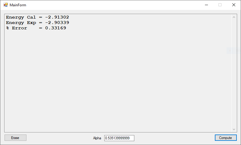
Using trial and error we calculate Alpha as: 0.535139999999
public double Integrate(double[] lower, double[] upper, double[] alpha,
            Func<double[], double[], double> f, int n, int[] steps)
        {
            double p = 1;
            double[] h = new double[n];
            double[] h2 = new double[n];
            double[] s = new double[n];
            double[] t = new double[n];
            double[] x = new double[n];
            double[] w = new double[n];

            for (int i = 0; i < n; i++)
            {
                h[i] = (upper[i] - lower[i]) / steps[i];
                h2[i] = 2.0 * h[i];
            }

            for (int i = 0; i < n; i++)
            {
                for (int j = 0; j < n; j++)
                    x[j] = lower[j];

                x[i] = lower[i] + h[i];

                for (int j = 1; j < steps[i]; j += 2)
                {
                    s[i] += f(x, alpha);
                    x[i] += h2[i];
                }

                for (int j = 0; j < n; j++)
                    x[j] = lower[j];

                x[i] = lower[i] + h2[i];

                for (int j = 2; j < steps[i]; j += 2)
                {
                    t[i] += f(x, alpha);
                    x[i] += h2[i];
                }

                w[i] = h[i] * (f(lower, alpha) + 4 * s[i] + 2 * t[i] + f(upper, alpha)) / 3.0;
            }

            for (int i = 0; i < n; i++)
                p *= w[i];

            return p;
        }
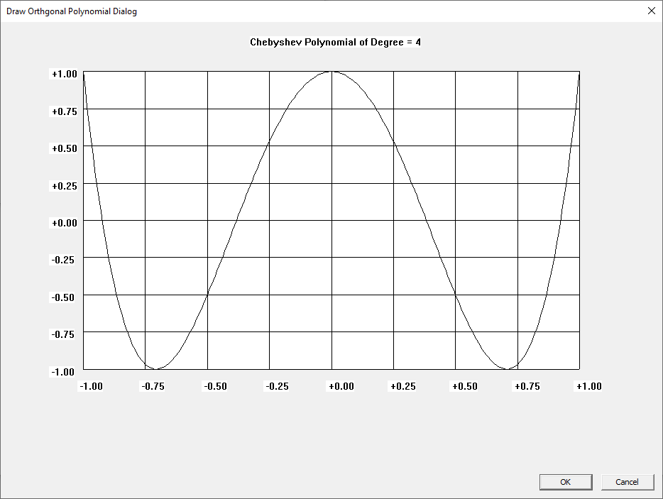
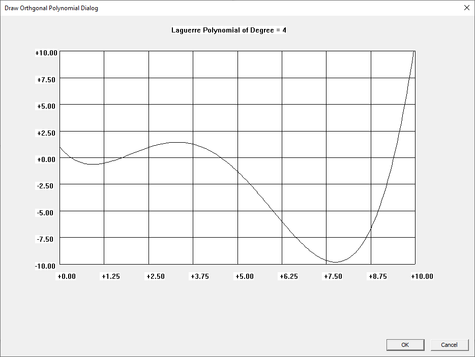
Win32 C Orthogonal Polynomials
I learned about the Laguerre and Legendre polynomials when I first read “Introduction to Quantum Mechanics” by Pauling and Wilson way back in the early 1970s. I later learned about the Chebyshev and other orthogonal polynomials. Beginning on March 30, 2015, I created yet another application to graph various orthogonal polynomials in C#. A few days ago, I wrote a Win32 C application to graph the Chebyshev, Laguerre, and Legendre orthogonal polynomials. At a later date, I will probably add Hermite and Jacobi polynomials.
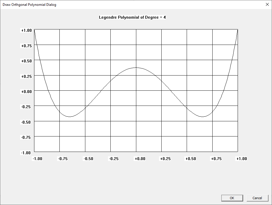
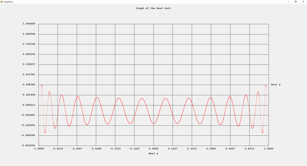
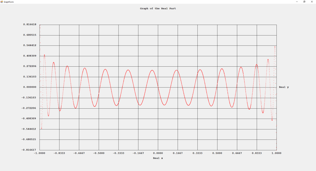
Three Term Recurrence Relations for the Legendre Functions by James Pate Williams, Jr.
bachelorthesis.dvi (uni-ulm.de)
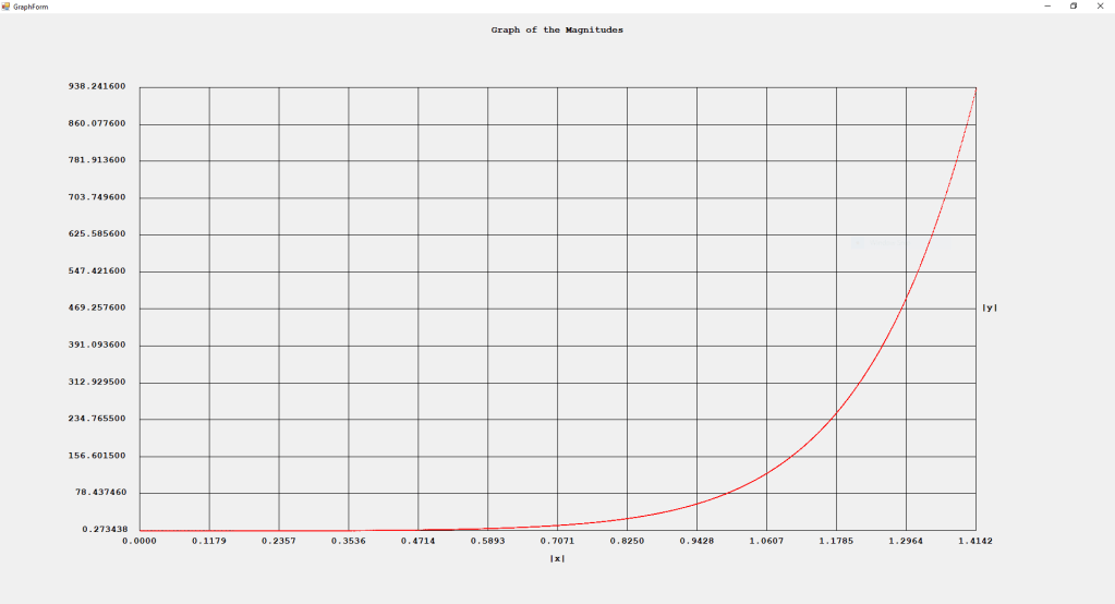
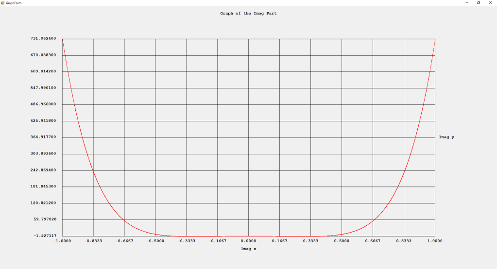
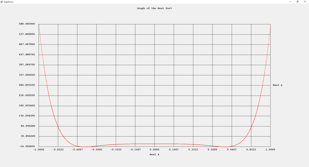
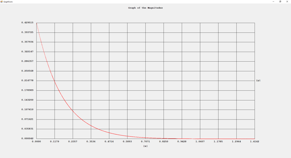
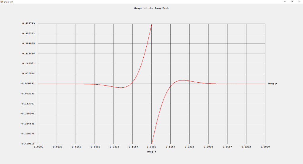
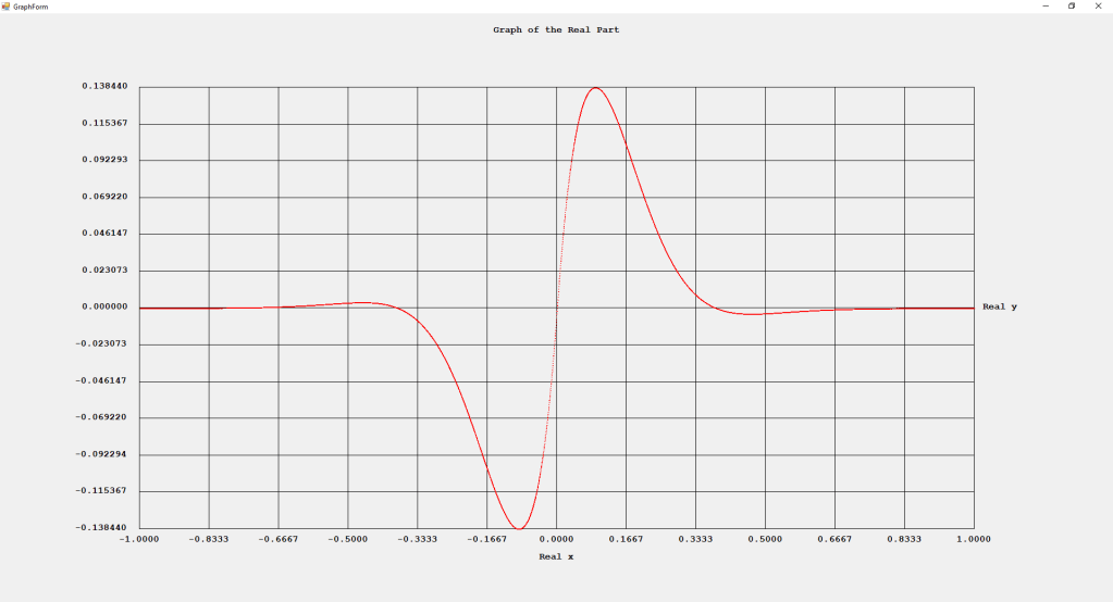
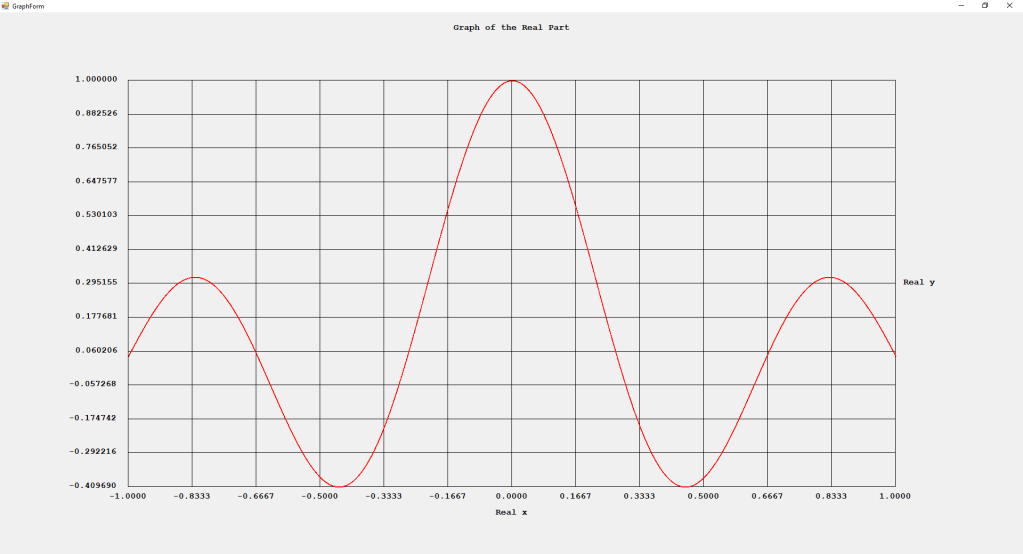
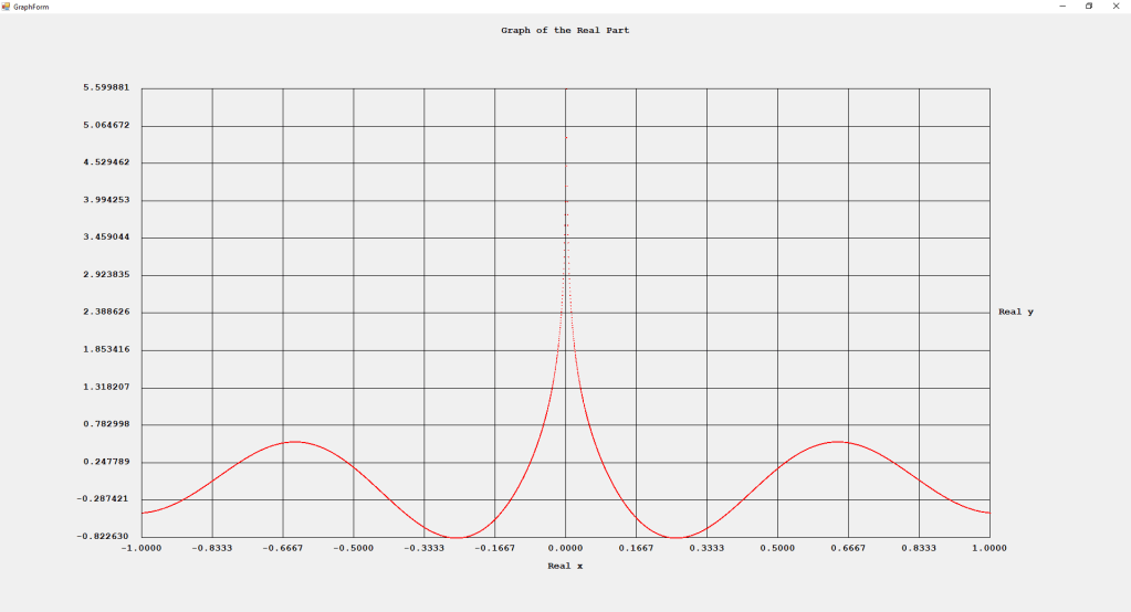
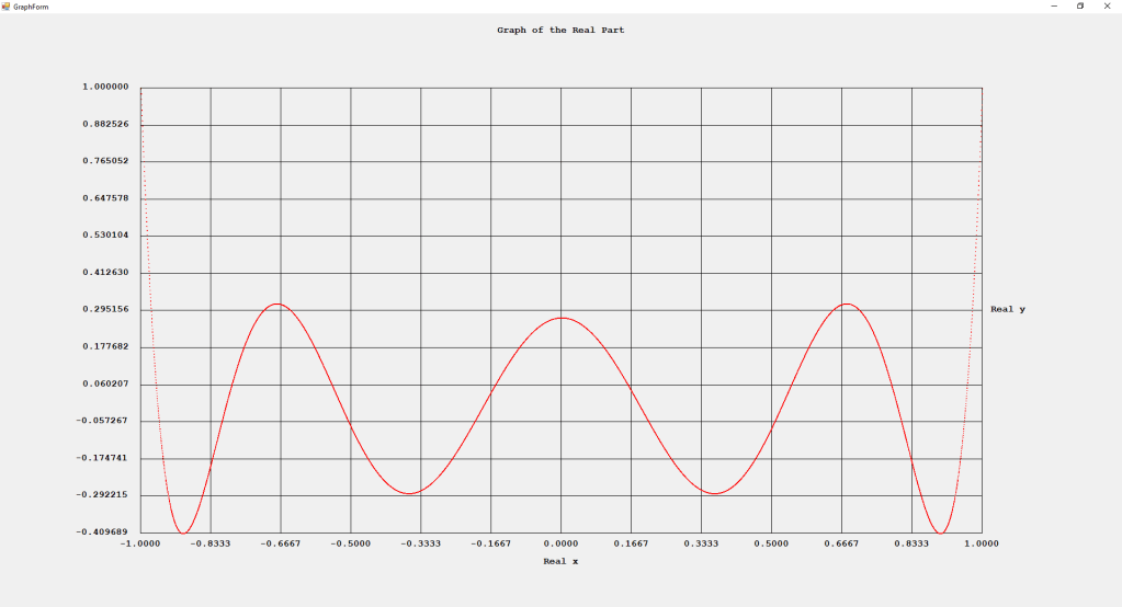
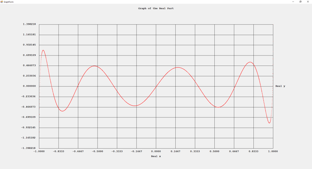
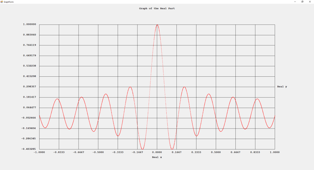
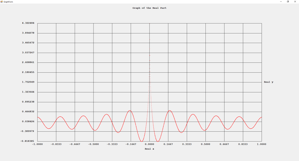
My implementations and additional graphs for the Legendre functions mentioned in the thesis cited in the preceding line and PDF. The Legendre polynomials, functions, and associated functions have many applications in quantum mechanics and other branches of applied and theoretical physics.

First Order Perturbation Calculation for the Helium Atom Ground State by James Pate Williams, Jr.
The first order perturbation calculation for the helium atom ground state is treated in detail in the textbook “Quantum Mechanics Third Edition” by Leonard I. Schiff pages 257 to 259. I offer a numerical algorithm for computing the electron-electron repulsion interaction which is analytically determined by Schiff and other scientists. Next is the graphical user interface for the application and its output.
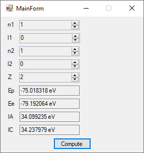
The Ep text box is the ground state energy as found by a first order perturbation computation. The Ee text box is the experimental ground state energy. The IA text box is the analytic electron-electron repulsion interaction determined by Schiff and other quantum mechanics researchers. The IC text box is my numerical contribution. All the energies are in electron volts.
The application source code are the next items in this blog.
