Old adage or aphorism: “A picture is worth a thousand words.”

Old adage or aphorism: “A picture is worth a thousand words.”
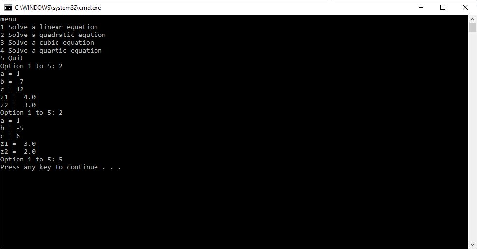
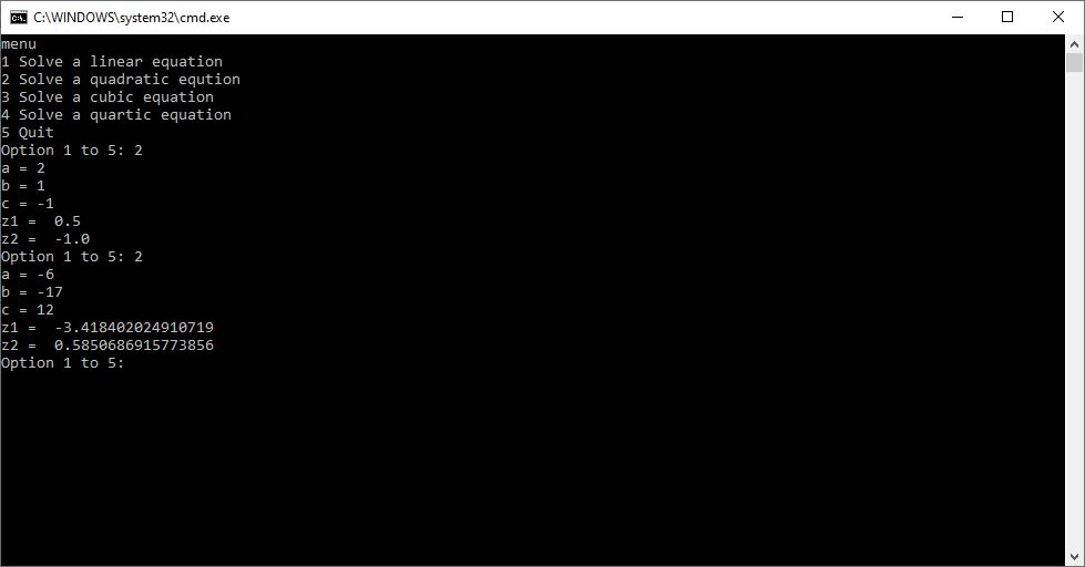
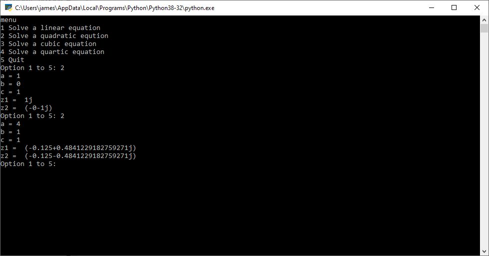
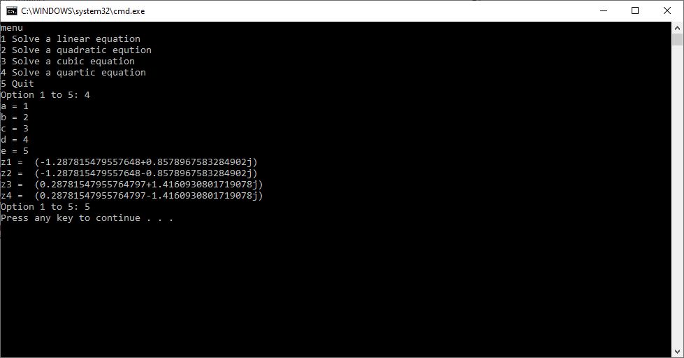
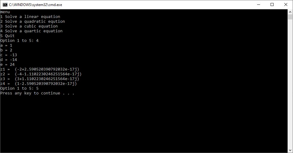
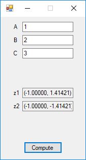
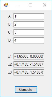
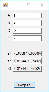
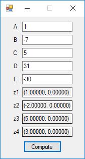
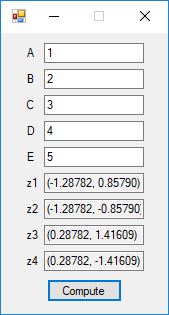
Back in 2015 I created a C# application to solve quadratic, cubic, and quartic equations which are of degrees 2, 3, and 4, respectively. Yesterday I successfully translated the C# to the Python console. I bench-marked my computer programs against the online calculators on the following website:
Cubic equation Calculator – High accuracy calculation (casio.com)
Quartic equation Calculator – High accuracy calculation (casio.com)
Here are my resulting Python outputs:

bachelorthesis.dvi (uni-ulm.de)
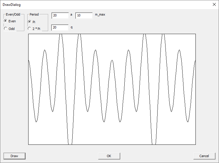
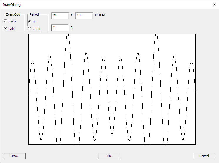
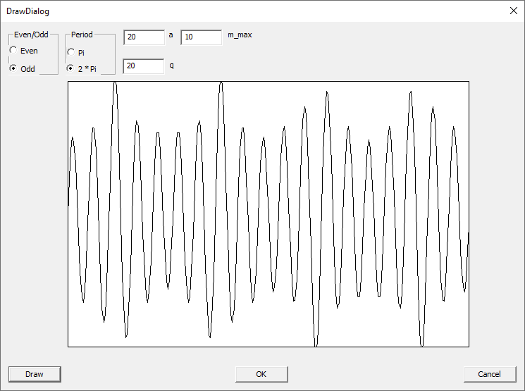
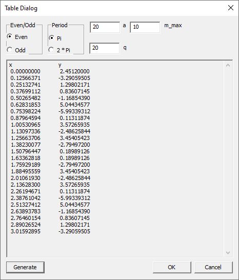
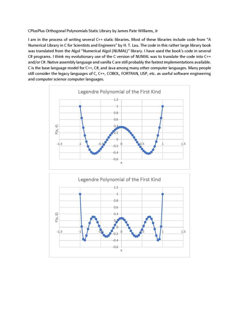
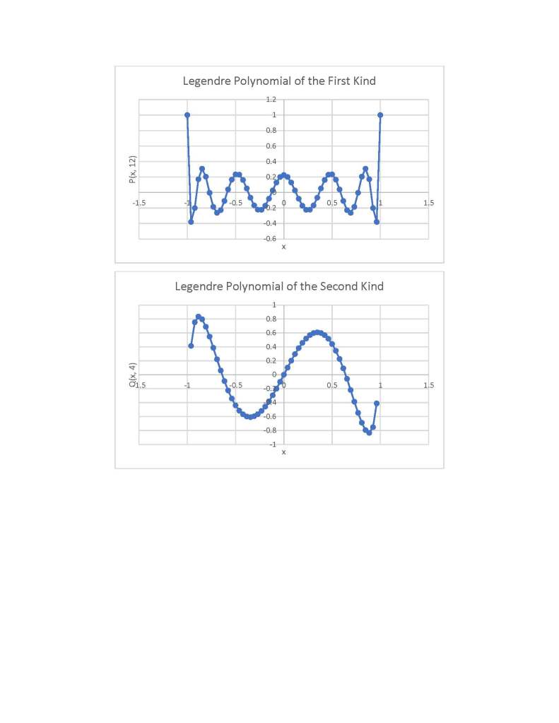
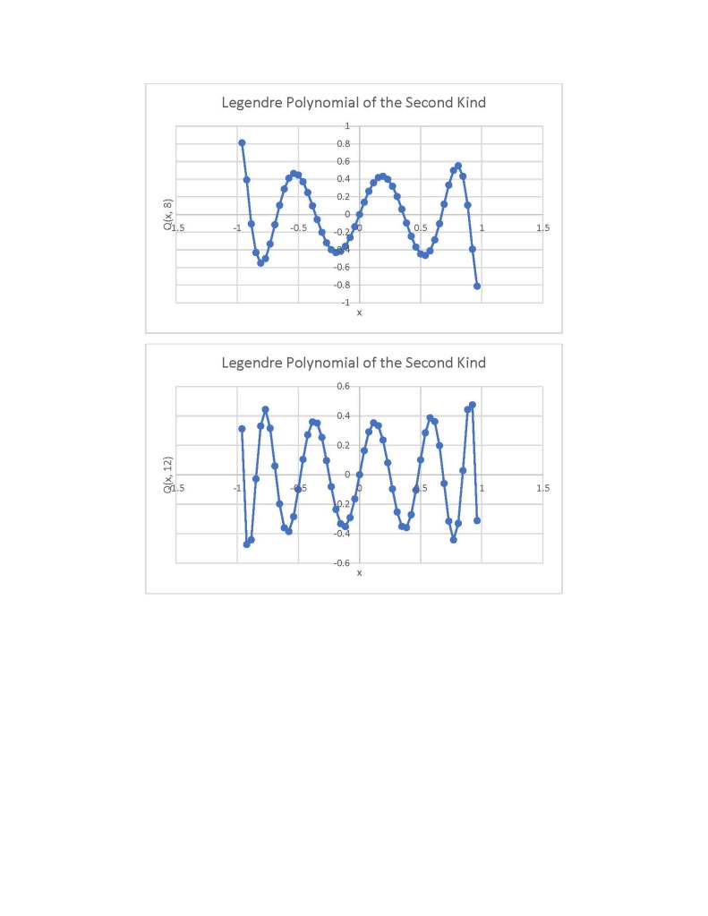
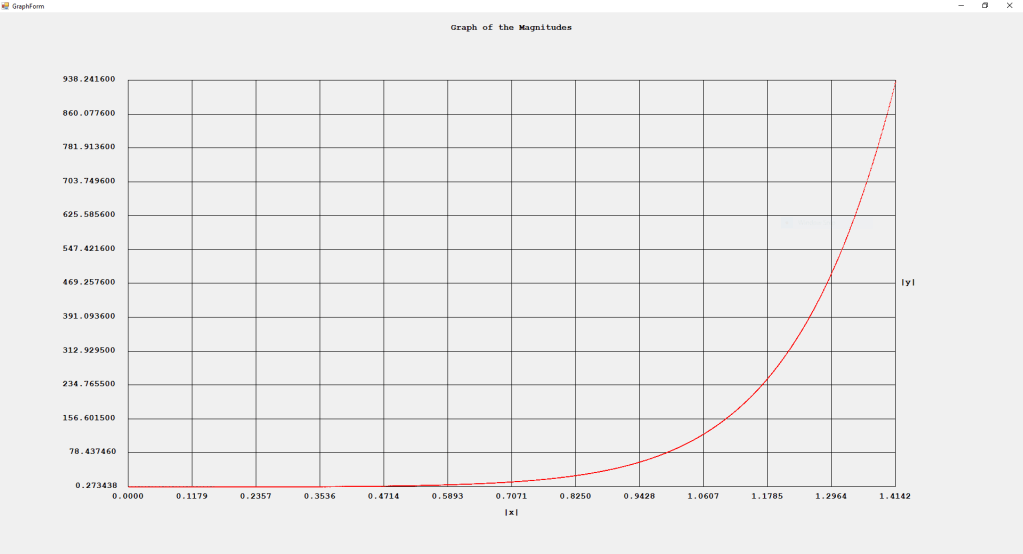
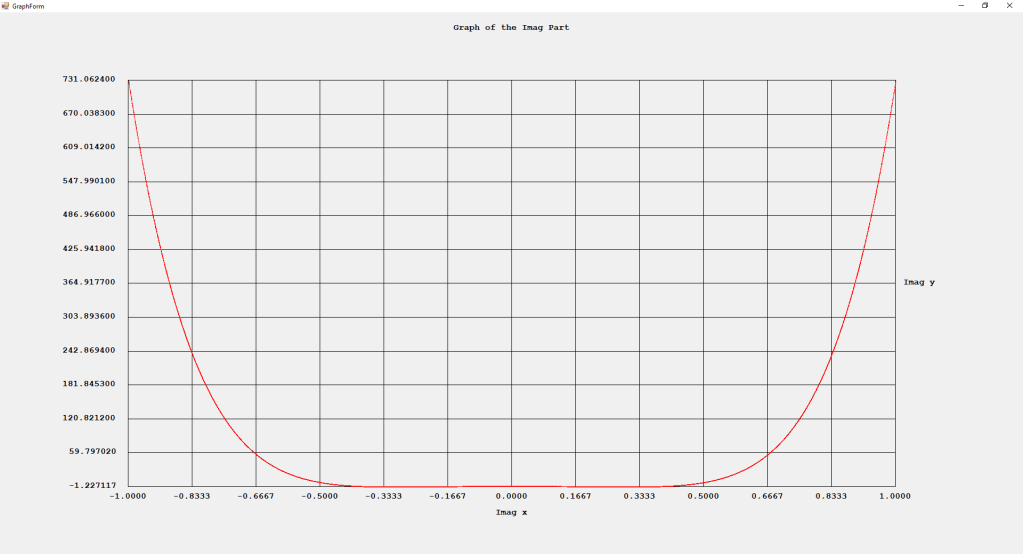
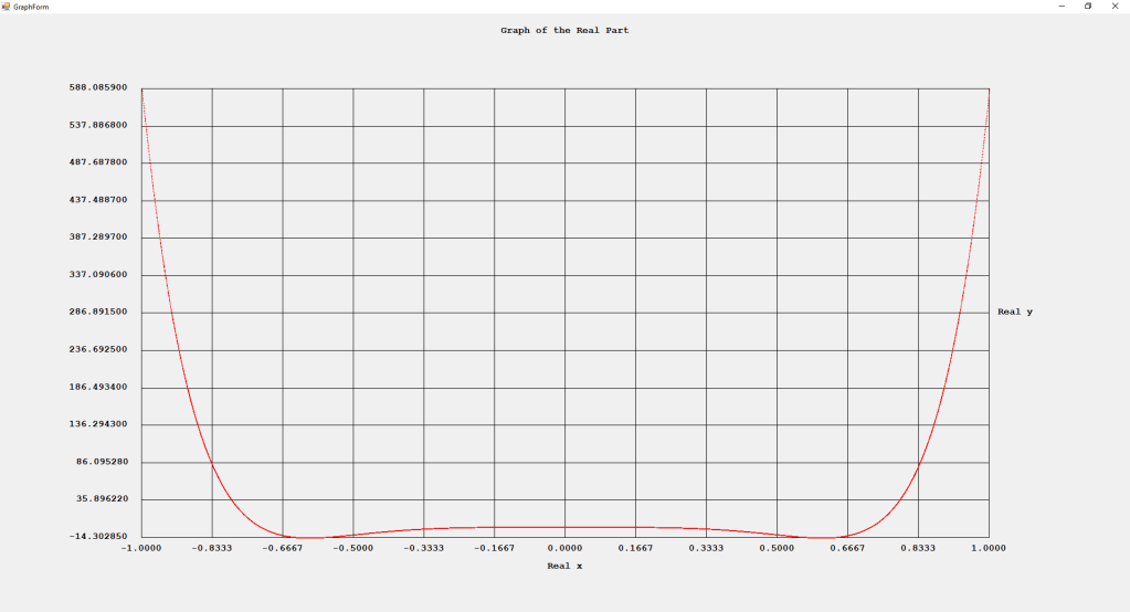
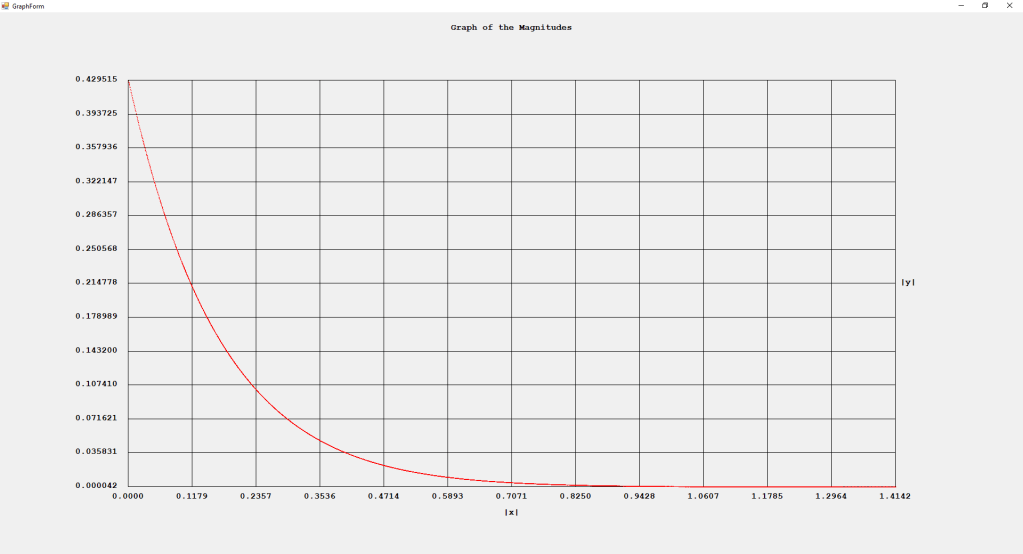
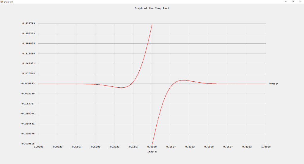
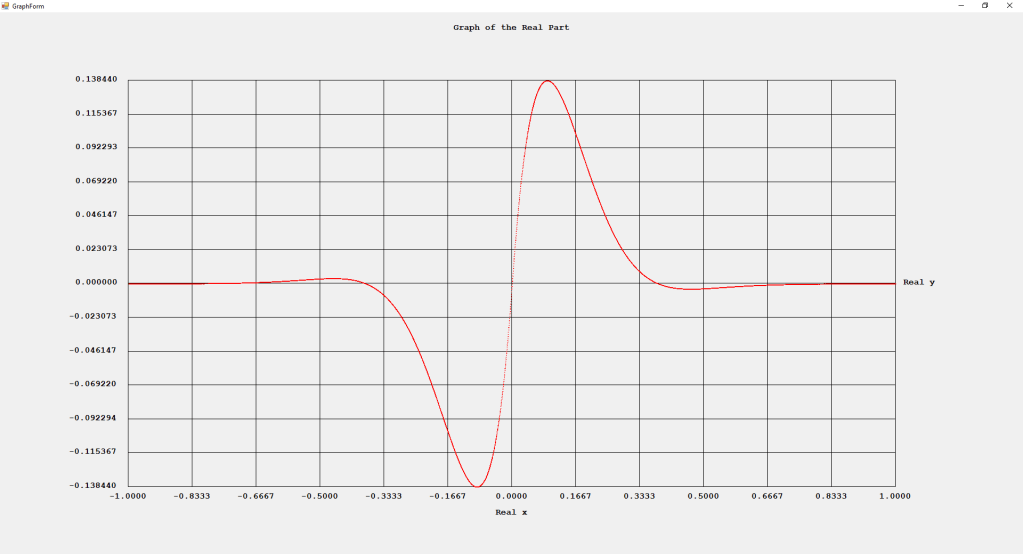
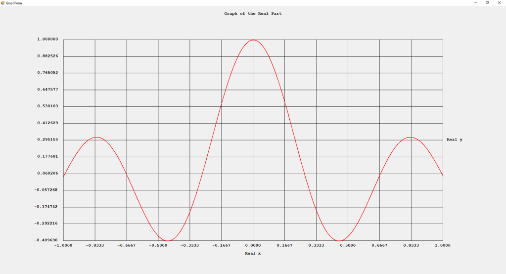
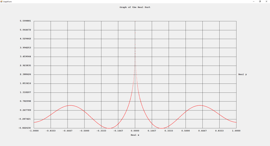
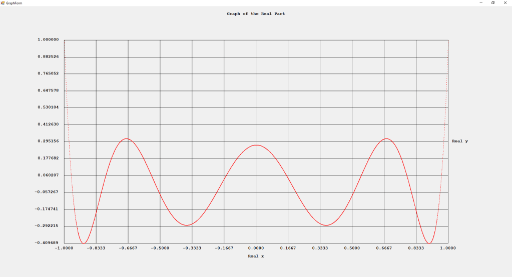
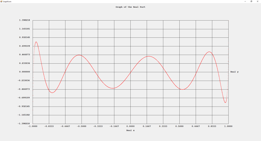
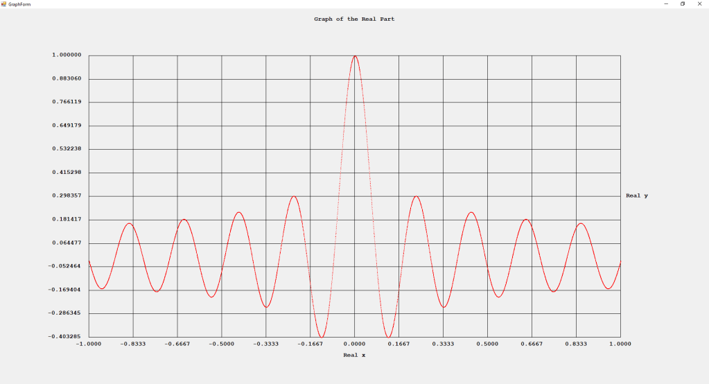
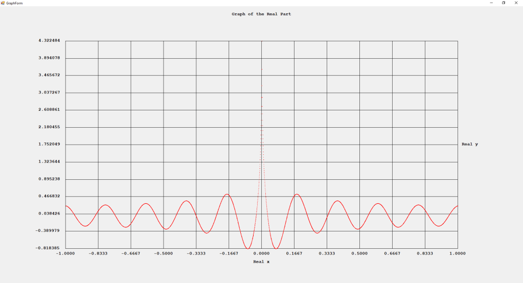
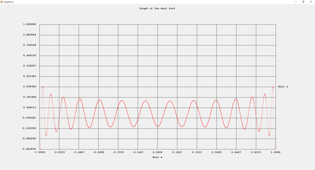
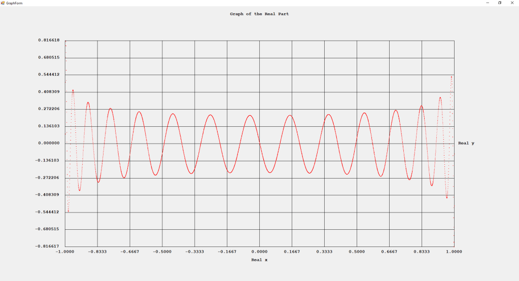
My implementations and additional graphs for the Legendre functions mentioned in the thesis cited in the preceding line and PDF. The Legendre polynomials, functions, and associated functions have many applications in quantum mechanics and other branches of applied and theoretical physics.
In my current return to my youthful dual interests in quantum chemistry and quantum mechanics that occupied much of my time in the 1960s, 1970s and 1980s, I am now using my knowledge of experimental numerical analysis. My interest in computer science and numerical analysis began in the summer of 1976 while I was a chemistry student at my local college namely LaGrange College in LaGrange, Georgia. As a child and teenager I was very interested in several disciplines of physics: classical mechanics, quantum mechanics, and the theories of special and general relativity. Later I added to my knowledge toolkit some tidbits of statistical mechanics and statistical thermodynamics.
This blog entry will explore the wonderful world of the hydrogenic atom which used to known by the moniker, hydrogen-like atom. The most well known isotope of hydrogen has one electron and one proton and its atomic number is 1 and it is sometimes denoted by the letter and numeral Z = 1. Of course, there are multiple other isotopes of hydrogen including deuterium (one proton and one neutron) and tritium (one proton and two neutrons). Hydrogen is the only atom whose wave functions both non-relativistic (see Erwin Schrödinger) and relativistic (view Paul Adrian Maurice Dirac) have analytic close formed solutions. Hydrogen is the most abundant chemical element on Earth and in the universe. The stars initially use a hydrogen plasma as a nuclear fuel to create more massive atomic ions and release massive amounts of nuclear fusion energy.
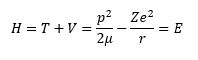
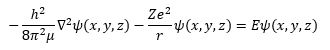
Way back in the 1920s Erwin Schrödinger decided to apply his work in wave hydrology to the newly found branch of physics known as quantum theory and quantum mechanics. From his work the branch of quantum mechanics known as wave quantum mechanics evolved. This branch was as important as another competing theory of quantum mechanics known as matrix quantum mechanics that was being concurrently developed by Werner Heisenberg. The key process in the derivation of a Schrödinger equation for any time independent scenario is to apply the first quantization rules to a valid classical Hamiltonian. The classical Hamiltonian is the total energy of a system and is the sum of the kinetic energy and the potential energy. The classical Hamiltonian for the hydrogen-like atom is shown in equation (1).
The first quantization rule is to apply the conversion from a classical momentum vector to a momentum quantum mechanical operator using the equation (2).
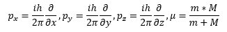
The lower case m is the mass of the electron and the upper case M is the mass of the atomic nucleus which is the Z times the proton mass plus the number of neutrons times the neutron mass. The Greek letter mu is the reduced mass of the hydrogen-like system. The italic i is the imaginary unit that is the square root of the number -1. The transcendental number pi is represented by the Greek letter pi and has the truncated real number value of 3.1415926535897932384626433832795. Schrödinger plugged Equation (2) into Equation (1) and found a three-dimensional Cartesian coordinate second order partial differential equation (3) that used the operator discovered by the mathematician Laplace.
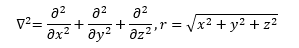
In equation (4) the first partial differential operator is the Laplace operator which is the vector inner product of the three-dimensional Cartesian gradient operator from vector analysis. The scalar r in equation (4) is the Euclidean distance from the electron to the nucleus. The Greek letter psi (“pitchfork”) in equation (3) is the illustrious and elusive wave function.
The first thing that struck Schrödinger was that the equation (3) that he derived by much thought was unfortunately not a separable partial differential equation in three-dimensional Cartesian coordinates, however, he next applied a coordinate coordinate transformation from three-dimensional Cartesian coordinates to three dimensional spherical polar equations specified by the equations in the following PDF with some derivations.
The wave function for the hydrogen-like atom is dependent on the associated Laguerre polynomials and the spherical harmonics that dependent upon the associated Legendre functions.
https://mathworld.wolfram.com/AssociatedLaguerrePolynomial.html
https://www.sciencedirect.com/topics/mathematics/associated-legendre-function
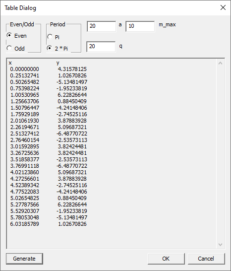
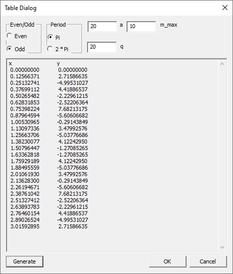
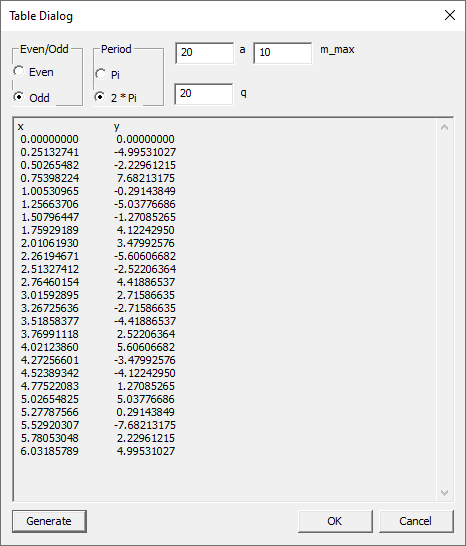
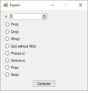
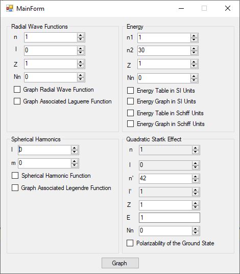
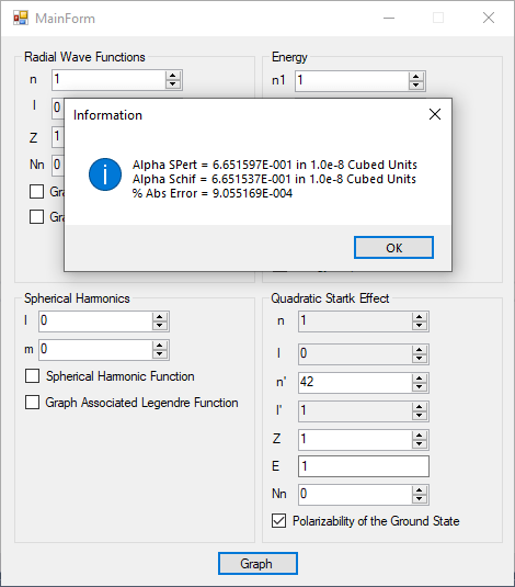
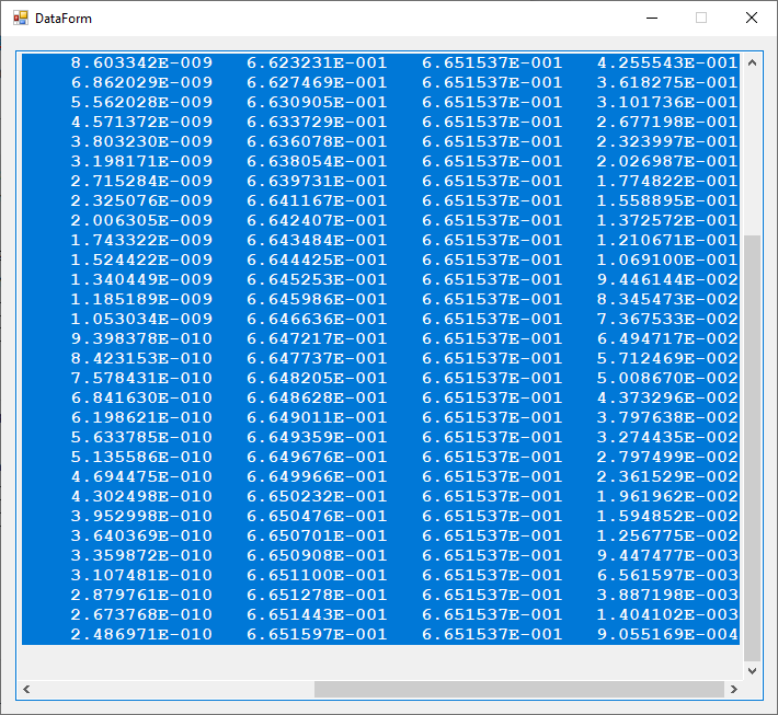
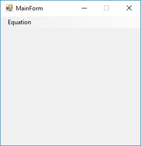
I created a useful C# desktop application that allows some graphical exploration of the hydrogen-like atom. Here is the graphical user interface.
The PDF file below are graphs for the radial wave functions for the hydrogen-like atom for n = 1 to 8 which are the s-orbitals.
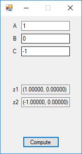
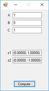
We designed and implemented quadratic formula, cubic formula, and quartic formula solvers using the formulas in the Wikipedia articles:
https://en.wikipedia.org/wiki/Quadratic_formula
https://en.wikipedia.org/wiki/Cubic_function
https://en.wikipedia.org/wiki/Quartic_function
We tested our C# implementation against:
https://keisan.casio.com/exec/system/1181809415
http://www.wolframalpha.com/widgets/view.jsp?id=3f4366aeb9c157cf9a30c90693eafc55
https://keisan.casio.com/exec/system/1181809416
Here are screenshots of the C# application:
C# source code files for the application:
